Download
1 / 65
710 likes | 801 Views
Explore the science of color, light, and human vision in multimedia systems. Learn about color models, spectral sensitivity of the eye, and image formation processes. Dive into Sir Isaac Newton's experiments and examine the role of cones and rods in vision.

E N D
Iran University of Science and Technology,E-Learing Center, Fall 2008 (1387) Chapter 4Color in Image and Video 4.1 Color Science 4.2 Color Models in Images 4.3 Color Models in Video
4.1 Color Science • Light and Spectra • • Light is an electromagnetic wave. Its color is characterized by the wavelength content of the light. • (a) Laser light consists of a single wavelength: e.g., a ruby laser produces a bright, scarlet-red beam. • (b) Most light sources produce contributions over many wavelengths. • (c) However, humans cannot detect all light, just contributions that fall in the “visible wavelengths”. • (d) Short wavelengths produce a blue sensation, long wavelengths produce a red one. • • Spectrophotometer: device used to measure visible light, by reflecting light from a diffraction grating (a ruled surface) that spreads out the different wavelengths. Multimedia Systems (eadeli@iust.ac.ir)
• Figure 4.1 shows the phenomenon that white light contains all the colors of a rainbow. • • Visible light is an electromagnetic wave in the range 400 nm to 700 nm (where nm stands for nanometer, 10−9 meters). Fig. 4.1: Sir Isaac Newton’s experiments. Multimedia Systems (eadeli@iust.ac.ir)
• Fig. 4.2 shows the relative power in each wavelength interval for typical outdoor light on a sunny day. This type of curve is called a Spectral Power Distribution (SPD) or a spectrum. • • The symbol for wavelength is λ. This curve is called E(λ). • Fig. 4.2: Spectral power distribution of daylight. Multimedia Systems (eadeli@iust.ac.ir)
Human Vision • • The eye works like a camera, with the lens focusing an image onto the retina (upside-down and left-right reversed). • • The retina consists of an array of rods and three kinds of cones. • • The rods come into play when light levels are low and produce a image in shades of gray (“all cats are gray at night!”). • • For higher light levels, the cones each produce a signal. Because of their differing pigments, the three kinds of cones are most sensitive to red (R), green (G), and blue (B) light. • • It seems likely that the brain makes use of differences R-G, G-B, and B-R, as well as combining all of R, G, and B into a high-light-level achromatic channel. Multimedia Systems (eadeli@iust.ac.ir)
Spectral Sensitivity of the Eye • • The eye is most sensitive to light in the middle of the visible spectrum. • • The sensitivity of our receptors is also a function of wavelength (Fig. 4.3 below). • • The Blue receptor sensitivity is not shown to scale because it is much smaller than the curves for Red or Green — Blue is a late addition, in evolution. • – Statistically, Blue is the favorite color of humans, regardless of nationality — perhaps for this reason: Blue is a latecomer and thus is a bit surprising! • • Fig. 4.3 shows the overall sensitivity as a dashed line — this important curve is called the luminous-efficiency function. • – It is usually denoted V (λ) and is formed as the sum of the response • curves for Red, Green, and Blue. Multimedia Systems (eadeli@iust.ac.ir)
• The rod sensitivity curve looks like the luminous-efficiency function V (λ) but is shifted to the red end of the spectrum. • • The achromatic channel produced by the cones is approximately proportional to 2R+G+B/20. • Fig. 4.3: R,G, and B cones, and Luminous Efficiency curve V(λ). Multimedia Systems (eadeli@iust.ac.ir)
• These spectral sensitivity functions are usually denoted by letters other than “R,G,B”; here let’s use a vector function q(λ), with components • q (λ) = (qR(λ), qG(λ), qB(λ))T (4.1) • • The response in each color channel in the eye is proportional to the number of neurons firing. • • A laser light at wavelength λ would result in a certain number of neurons firing. An SPD is a combination of single-frequency lights (like “lasers”), so we add up the cone responses for all wavelengths, weighted by the eye’s relative response at that wavelength. Multimedia Systems (eadeli@iust.ac.ir)
• We can succinctly write down this idea in the form of an integral: • R = ∫E(λ) qR(λ) dλ • G = ∫E(λ) qG(λ) dλ • B = ∫E(λ) qB(λ) dλ (4.2) Multimedia Systems (eadeli@iust.ac.ir)
Image Formation • • Surfaces reflect different amounts of light at different wavelengths, and dark surfaces reflect less energy than light surfaces. • • Fig. 4.4 shows the surface spectral reflectance from (1) orange sneakers and (2) faded blue jeans. The reflectance function is denoted S(λ). Multimedia Systems (eadeli@iust.ac.ir)
Fig. 4.4: Surface spectral reflectance functions S(λ) for objects. Multimedia Systems (eadeli@iust.ac.ir)
• Image formation is thus: • – Light from the illuminant with SPD E(λ) impinges on a • surface, with surface spectral reflectance function S(λ), is • reflected, and then is filtered by the eye’s cone functions • q (λ). • – Reflection is shown in Fig. 4.5 below. • – The function C(λ) is called the color signal and consists • of the product of E(λ), the illuminant, times S(λ), the • reflectance: • C(λ) = E(λ) S(λ). Multimedia Systems (eadeli@iust.ac.ir)
Fig. 4.5: Image formation model. Multimedia Systems (eadeli@iust.ac.ir)
• The equations that take into account the image formation model are: • R = ∫E(λ) S(λ) qR(λ) dλ • G = ∫E(λ) S(λ) qG(λ) dλ • B = ∫E(λ) S(λ) qB(λ) dλ (4.3) Multimedia Systems (eadeli@iust.ac.ir)
Camera Systems • • Camera systems are made in a similar fashion; a studio quality camera has three signals produced at each pixel location (corresponding to a retinal position). • • Analog signals are converted to digital, truncated to integers, and stored. If the precision used is 8-bit, then the maximum value for any of R,G,B is 255, and the minimum is 0. • • However, the light entering the eye of the computer user is that which is emitted by the screen—the screen is essentially a self-luminous source. Therefore we need to know the light E(λ) entering the eye. Multimedia Systems (eadeli@iust.ac.ir)
Gamma Correction • • The light emitted is in fact roughly proportional to the voltage raised to a power; this power is called gamma, with symbol γ. • (a) Thus, if the file value in the red channel is R, the screen emits light proportional to Rγ, with SPD equal to that of the red phosphor paint on the screen that is the target of the red channel electron gun. The value of gamma is around 2.2. • (b) It is customary to append a prime to signals that are gamma-corrected by raising to the power (1/γ) before transmission. Thus we arrive at linear signals: • R → R′ = R1/γ ⇒ (R′)γ → R (4.4) Multimedia Systems (eadeli@iust.ac.ir)
• Fig. 4.6(a) shows light output with no gamma-correction applied. We see that darker values are displayed too dark. This is also shown in Fig. 4.7(a), which displays a linear ramp from left to right. • • Fig. 4.6(b) shows the effect of pre-correcting signals by applying the power law R1/γ; it is customary to normalize voltage to the range [0,1]. Multimedia Systems (eadeli@iust.ac.ir)
Fig. 4.6: (a): Effect of CRT on light emitted from screen (voltage is normalized to range 0..1). (b): Gamma correction of signal. Multimedia Systems (eadeli@iust.ac.ir)
• The combined effect is shown in Fig. 4.7(b). Here, a ramp is shown in 16 steps from gray-level 0 to gray-level 255. • Fig. 4.7: (a): Display of ramp from 0 to 255, with no gamma correction. (b): Image with gamma correction applied Multimedia Systems (eadeli@iust.ac.ir)
Color-Matching Functions • • Even without knowing the eye-sensitivity curves of Fig.4.3, a technique evolved in psychology for matching a combination of basic R, G, and B lights to a given shade. • • The particular set of three basic lights used in an experiment are called the set of color primaries. • • To match a given color, a subject is asked to separately adjust the brightness of the three primaries using a set of controls until the resulting spot of light most closely matches the desired color. • • The basic situation is shown in Fig.4.8. A device for carrying out such an experiment is called a colorimeter. Multimedia Systems (eadeli@iust.ac.ir)
Fig. 4.8: colorimeter experiment. Multimedia Systems (eadeli@iust.ac.ir)
• The amounts of R, G, and B the subject selects to match each single-wavelength light forms the color-matching curves. These are denoted and are shown in Fig. 4.9. • Fig. 4.9: CIE RGB color-matching functions . Multimedia Systems (eadeli@iust.ac.ir)
CIE Chromaticity Diagram • • Since the color-matching curve has a negative lobe, a set of fictitious primaries were devised that lead to color-matching functions with only positives values. • (a) The resulting curves are shown in Fig. 4.10; these are usually referred to as the color-matching functions. • (b) They are a 3 × 3 matrix away from curves, and are denoted . • (c) The matrix is chosen such that the middle standard color-matching function exactly equals the luminous-efficiency curve V(λ) shown in Fig. 4.3. Multimedia Systems (eadeli@iust.ac.ir)
International Commission on Illumination (usually known as the CIE for its French name Commission internationale de l'éclairage) • Fig. 4.10: CIE standard XYZ color-matching functions . Multimedia Systems (eadeli@iust.ac.ir)
• For a general SPD E(λ), the essential “colorimetric” information required to characterize a color is the set of tristimulus values X, Y, Z defined in analogy to (Eq. 4.2) as (Y == luminance): • (4.6) • • 3D data is difficult to visualize, so the CIE devised a 2D diagram based on the values of (X, Y, Z) triples implied by the curves in Fig. 4.10. Multimedia Systems (eadeli@iust.ac.ir)
• We go to 2D by factoring out the magnitude of vectors (X, Y, Z); we could divide by , but instead we divide by the sum X + Y + Z to make the chromaticity: • x = X/(X +Y +Z) • y = Y/(X +Y +Z) • z = Z/(X +Y +Z) (4.7) • • This effectively means that one value out of the set (x, y, z) is redundant since we have • (4.8) • so that • z = 1 − x − y (4.9) Multimedia Systems (eadeli@iust.ac.ir)
• Effectively, we are projecting each tristimulus vector (X, Y, Z) onto the plane connecting points (1, 0, 0), (0, 1, 0), and (0, 0, 1). • • Fig. 4.11 shows the locus of points for monochromatic light • Fig. 4.11: CIE chromaticity diagram. Multimedia Systems (eadeli@iust.ac.ir)
The color matching curves each add up to the same value — the area under each curve is the same for each of . • (b) For an E(λ) = 1 for all λ, — an “equi-energy white light”— chromaticity values are (1/3, 1/3). Fig. 4.11 displays a typical actual white point in the middle of the diagram. • (c) Since x, y ≤ 1 and x + y ≤ 1, all possible chromaticity values lie below the dashed diagonal line in Fig. 4.11. Multimedia Systems (eadeli@iust.ac.ir)
• The human eye has three types of color sensors. • A full plot of all visible colors is a three-dimensional figure. • The concept of color can be divided into two parts: brightness and chromaticity. • The CIE XYZ color space: • Y parameter: a measure of the brightness or luminance of a color. • The chromaticity of a color: two derived parameters x and y. • CIE xyY color space. Multimedia Systems (eadeli@iust.ac.ir)
Color Monitor Specifications • • Color monitors are specified in part by the white point chromaticity that is desired if the RGB electron guns are all activated at their highest value (1.0, if we normalize to [0,1]). • • We want the monitor to display a specified white when R′=G′=B′=1. • • There are several monitor specifications in current use (Table 4.1). Multimedia Systems (eadeli@iust.ac.ir)
Table 4.1: Chromaticities and White Points of Monitor Specifications Multimedia Systems (eadeli@iust.ac.ir)
Out-of-Gamut colors • • For any (x, y) pair we wish to find that RGB triple giving the specified (x, y, z): We form the z values for the phosphors, via z = 1 − x − y and solve for RGB from the phosphor chromaticities. • • We combine nonzero values of R, G, and B via • (4.10) Multimedia Systems (eadeli@iust.ac.ir)
• If (x, y) [color without magnitude] is specified, instead of derived as above, we have to invert the matrix of phosphor (x, y, z) values to obtain RGB. • • What do we do if any of the RGB numbers is negative? — that color, visible to humans, is out-of-gamut for our display. • 1. One method: simply use the closest in-gamut color available, as in Fig. 4.13. • 2. Another approach: select the closest complementary color. Multimedia Systems (eadeli@iust.ac.ir)
Fig. 4.13: Approximating an out-of-gamut color by an in-gamut one. The out-of-gamut color shown by a triangle is approximated by the intersection of (a) the line from that color to the white point with (b) the boundary of the device color gamut. Multimedia Systems (eadeli@iust.ac.ir)
• Grassman’s Law: (Additive) color matching is linear. This means that if we match color1 with a linear combinations of lights and match color2 with another set of weights, the combined color color1+color2 is matched by the sum of the two sets of weights. • • Additive color results from self-luminous sources, such as lights projected on a white screen, or the phosphors glowing on the monitor glass. (Subtractive color applies for printers, and is very different). • • Fig. 4.13 above shows the triangular gamut for the NTSC system, drawn on the CIE diagram — a monitor can display only the colors inside a triangular gamut. Multimedia Systems (eadeli@iust.ac.ir)
Gamut of the CIE RGB primaries and location of primaries on the CIE 1931 xy chromaticity diagram. Multimedia Systems (eadeli@iust.ac.ir)
White Point Correction • • Problems: • One deficiency in what we have done so far is that we need to be able to map tristimulus values XYZ to device RGBs including magnitude, and not just deal with chromaticity xyz. • (b) Table 4.1 would produce incorrect values: • – E.g., consider the SMPTE specifications. Setting R = G = B = 1 results in a value of X that equals the sum of the x values, or 0.630 + 0.310 + 0.155, which is 1.095. Similarly the Y and Z values come out to 1.005 and 0.9. Now, dividing by (X + Y + Z) this results in a chromaticity of (0.365, 0.335), rather than the desired values of (0.3127, 0.3291). Multimedia Systems (eadeli@iust.ac.ir)
• To correct both problems, first take the white point magnitude of Y as unity: • Y (white point) = 1 (4.11) • • Now we need to find a set of three correction factors such that if the gains of the three electron guns are multiplied by these values we get exactly the white point XYZ value at R = G = B = 1. Multimedia Systems (eadeli@iust.ac.ir)
• Suppose the matrix of phosphor chromaticitiesxr, xg, ... Etc. in Eq. (4.10) is called M . We can express the correction as a diagonal matrix D = diag(d1, d2, d3) such that • XYZwhite ≡ MD (1, 1, 1)T (4.12) • • For the SMPTE specification, we have (x, y, z) = (0.3127, 0.3291, 0.3582) or, dividing by the middle value — XYZwhite = (0.95045, 1 , 1.08892). We note that multiplying D by (1, 1, 1)T just gives (d1, d2, d3)T so we end up with an equation specifying (d1, d2, d3)T: • (4.13) Multimedia Systems (eadeli@iust.ac.ir)
• Inverting, with the new values XYZwhite specified as above, we arrive at • (d1, d2, d3) = (0.6247, 1.1783, 1.2364) (4.14) • These are large correction factors. Multimedia Systems (eadeli@iust.ac.ir)
XYZ to RGB Transform • • Now the 3 × 3 transform matrix from XYZ to RGB is taken to be • T = M D (4.15) • even for points other than the white point: • (4.16) • • For the SMPTE specification, we arrive at: • (4.17) • • Written out, this reads: • (4.18) Multimedia Systems (eadeli@iust.ac.ir)
Transform with Gamma Correction • • Instead of linear R,G,B we usually have nonlinear, gamma corrected R′, G′, B′ (produced by a camcorder or digital camera). • • To transform XY Z to RGB, calculate the linear RGB required, by inverting Eq. (4.16) above; then make nonlinear signals via gamma correction. • • Nevertheless this is not often done as stated. Instead, the equation for the Y value is used as is, but applied to nonlinear signals. • (a) The only concession to accuracy is to give the new name Y ′ to this new Y value created from R′, G′, B′. • (b) The significance of Y ′ is that it codes a descriptor of brightness for the pixel in question. Multimedia Systems (eadeli@iust.ac.ir)
• Following the procedure outlined above, but with the values in Table 4.1 for NTSC, we arrive at the following transform: • (4.19) • • Thus, coding for nonlinear signals begins with encoding the nonlinear-signal correlate of luminance: • Y ′ = 0.299·R′+0.587·G′+0.114·B′ (4.20) Multimedia Systems (eadeli@iust.ac.ir)
L*a*b* (CIELAB) color Model • • Weber’s Law: Equally-perceived differences are proportional to magnitude. The more there is of a quantity, the more change there must be to perceive a difference. • • A rule of thumb for this phenomenon states that equally-perceived changes must be relative — changes are about equally perceived if the ratio of the change is the same, whether for dark or bright lights, etc. • • Mathematically, with intensity I, change is equally perceived so long as the change is a constant. If it’s quiet, we can hear a small change in sound. If there is a lot of noise, to experience the same difference the change has to be of the same proportion. Multimedia Systems (eadeli@iust.ac.ir)
• For human vision, the CIE arrived at a different version of this kind of rule — CIELAB space. What is being quantified in this space is differences perceived in color and brightness. • • Fig. 4.14 shows a cutaway into a 3D solid of the coordinate space associated with this color difference metric. Multimedia Systems (eadeli@iust.ac.ir)
Fig. 4.14: CIELAB model. Multimedia Systems (eadeli@iust.ac.ir)
• CIELAB: • (4.21) • (4.22) • with Xn, Yn, Zn the XYZ values of the white point. Auxiliary definitions are: Multimedia Systems (eadeli@iust.ac.ir)
More Color Coordinate Schemes • • Beware: gamma correction or not is usually ignored. • • Schemes include: • a) CMY — Cyan (C), Magenta (M) and Yellow (Y) color model; • b) HSL — Hue, Saturation and Lightness; • c) HSV — Hue, Saturation and Value; • d) HSI — Hue, Saturation and Intensity; • e) HCI — C=Chroma; • f) HVC — V=Value; • g) HSD — D=Darkness. Multimedia Systems (eadeli@iust.ac.ir)
4.2 Color Models in Images • • Colors models and spaces used for stored, displayed, and printed images. • • RGB Color Model for CRT Displays • 1. We expect to be able to use 8 bits per color channel for color that is accurate enough. • 2. However, in fact we have to use about 12 bits per channel to avoid an aliasing effect in dark image areas — contour bands that result from gamma correction. • 3. For images produced from computer graphics, we store integers proportional to intensity in the frame buffer. So should have a gamma correction LUT between the frame buffer and the CRT. • 4. If gamma correction is applied to floats before quantizing to integers, before storage in the frame buffer, then in fact we can use only 8 bits per channel and still avoid contouring artifacts. Multimedia Systems (eadeli@iust.ac.ir)