Download
1 / 85
910 likes | 1.41k Views
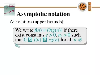
Intuition for Asymptotic Notation. Big-Oh f(n) is O(g(n)) if f(n) is asymptotically less than or equal to g(n) big-Omega f(n) is (g(n)) if f(n) is asymptotically greater than or equal to g(n) big-Theta f(n) is (g(n)) if f(n) is asymptotically equal to g(n) little-oh

E N D
Intuition for Asymptotic Notation Big-Oh • f(n) is O(g(n)) if f(n) is asymptotically less than or equal to g(n) big-Omega • f(n) is (g(n)) if f(n) is asymptotically greater than or equal to g(n) big-Theta • f(n) is (g(n)) if f(n) is asymptotically equal to g(n) little-oh • f(n) is o(g(n)) if f(n) is asymptotically strictly less than g(n) little-omega • f(n) is (g(n)) if is asymptotically strictly greater than g(n)
Analysis of Merge-Sort • The height h of the merge-sort tree is O(log n) • at each recursive call we divide in half the sequence, • The overall amount or work done at the nodes of depth i is O(n) • we partition and merge 2i sequences of size n/2i • we make 2i+1 recursive calls • Thus, the total running time of merge-sort is O(n log n)
Tools: Recurrence Equation Analysis • The final step of merge-sort consists of merging two sorted sequences, each with n/2 elements. It takes at most bn steps, for some constant b. • Likewise, the basis case (n< 2) will take at b most steps. • Therefore, if we let T(n) denote the running time of merge-sort: • We can therefore analyze the running time of merge-sort by finding a closed form solution to the above equation. • That is, a solution that has T(n) only on the left-hand side.
The Recursion Tree • Draw the recursion tree for the recurrence relation and look for a pattern: Total time = bn + bn log n (last level plus all previous levels)
Iterative Substitution • In the iterative substitution, or “plug-and-chug,” technique, we iteratively apply the recurrence equation to itself and see if we can find a pattern: • Note that base, T(n)=b, case occurs when 2i=n. That is, i = log n. • So, • Thus, T(n) is O(n log n).
Guess-and-Test Method • In the guess-and-test method, we guess a closed form solution and then try to prove it is true by induction: • Guess: T(n) < cn log n. • Wrong: we cannot make this last line be less than cn log n
Guess-and-Test Method, Part 2 • Recall the recurrence equation: • Guess #2: T(n) < cn log2 n. • So, T(n) is O(n log2 n). • In general, to use this method, you need to have a good guess and you need to be good at induction proofs.
Master Method (Chapter 5) • Many recurrence equations have the form: • The Master Theorem:
Master Method, Example 1 • The form: • The Master Theorem: • Example: Solution: logba=2, so case 1 says T(n) is O(n2).
Master Method, Example 2 • The form: • The Master Theorem: • Example: Solution: logba=1, so case 2 says T(n) is O(n log2 n).
Master Method, Example 3 • The form: • The Master Theorem: • Example: Solution: logba=0, so case 3 says T(n) is O(n logn).
Master Method, Example 4 • The form: • The Master Theorem: • Example: Solution: logba=3, so case 1 says T(n) is O(n3).
Master Method, Example 5 • The form: • The Master Theorem: • Example: Solution: logba=2, so case 3 says T(n) is O(n3).
Master Method, Example 6 • The form: • The Master Theorem: • Example: (binary search) Solution: logba=0, so case 2 says T(n) is O(log n).
Master Method, Example 7 • The form: • The Master Theorem: • Example: (heap construction) Solution: logba=1, so case 1 says T(n) is O(n).
Iterative “Proof” of the Master Theorem • Using iterative substitution, let us see if we can find a pattern: • We then distinguish the three cases as • The first term is dominant • Each part of the summation is equally dominant • The summation is a geometric series
Case Study Priority Queue Sorting
A priority queue stores a collection of items An item is a pair(key, element) Main methods of the Priority Queue ADT insertItem(k, e)inserts an item with key k and element e removeMin()removes the item with smallest key and returns its element Priority Queue ADT
Sorting with a Priority Queue AlgorithmPQ-Sort(S, C) • Inputsequence S, comparator C for the elements of S • Outputsequence S sorted in increasing order according to C P priority queue with comparator C whileS.isEmpty () e S.remove (S.first ()) P.insertItem(e, e) whileP.isEmpty() e P.removeMin() S.insertLast(e) • We can use a priority queue to sort a set of comparable elements • Insert the elements one by one with a series of insertItem(e, e) operations • Remove the elements in sorted order with a series of removeMin() operations • The running time of this sorting method depends on the priority queue implementation
Implementation with an unsorted sequence Store the items of the priority queue in a list-based sequence, in arbitrary order Performance: insertItem takes O(1) time since we can insert the item at the beginning or end of the sequence removeMin, minKey and minElement take O(n) time since we have to traverse the entire sequence to find the smallest key Sequence-based Priority Queue
Selection-Sort • Selection-sort is the variation of PQ-sort where the priority queue is implemented with an unsorted sequence • Running time of Selection-sort: • Inserting the elements into the priority queue with ninsertItem operations takes O(n) time • Removing the elements in sorted order from the priority queue with nremoveMin operations takes time proportional to1 + 2 + …+ n • Selection-sort runs in O(n2) time
Implementation with a sorted sequence Store the items of the priority queue in a sequence, sorted by key Performance: insertItem takes O(n) time since we have to find the place where to insert the item removeMin, minKey and minElement take O(1) time since the smallest key is at the beginning of the sequence Sequence-based Priority Queue
Insertion-Sort • Insertion-sort is the variation of PQ-sort where the priority queue is implemented with a sorted sequence • Running time of Insertion-sort: • Inserting the elements into the priority queue with ninsertItem operations takes time proportional to1 + 2 + …+ n • Removing the elements in sorted order from the priority queue with a series of nremoveMin operations takes O(n) time • Insertion-sort runs in O(n2) time
2 5 6 9 7 Heaps and Priority Queues
A heap is a binary tree storing keys at its internal nodes and satisfying the following properties: Heap-Order: for every internal node v other than the root,key(v) key(parent(v)) Complete Binary Tree: let h be the height of the heap for i = 0, … , h - 1, there are 2i nodes of depth i at depth h- 1, the internal nodes are to the left of the external nodes The last node of a heap is the rightmost internal node of depth h- 1 What is a heap (§2.4.3) 2 5 6 9 7 last node
Height of a Heap (§2.4.3) • Theorem: A heap storing n keys has height O(log n) Proof: (we apply the complete binary tree property) • Let h be the height of a heap storing n keys • Since there are 2i keys at depth i= 0, … , h - 2 and at least one key at depth h - 1, we have n 1 + 2 + 4 + … + 2h-2 + 1 • Thus, n 2h-1 , i.e., h log n + 1 depth keys 0 1 1 2 h-2 2h-2 h-1 1
Heaps and Priority Queues • We can use a heap to implement a priority queue • We store a (key, element) item at each internal node • We keep track of the position of the last node (2, Sue) (5, Pat) (6, Mark) (9, Jeff) (7, Anna)
Method insertItem of the priority queue ADT corresponds to the insertion of a key k to the heap The insertion algorithm consists of three steps Find the insertion node z (the new last node) Store k at z and expand z into an internal node Restore the heap-order property (discussed next) 2 5 6 9 7 Insertion into a Heap (§2.4.3) z insertion node 2 5 6 z 9 7 1
Upheap • After the insertion of a new key k, the heap-order property may be violated • Algorithm upheap restores the heap-order property by swapping k along an upward path from the insertion node • Upheap terminates when the key k reaches the root or a node whose parent has a key smaller than or equal to k • Since a heap has height O(log n), upheap runs in O(log n) time 2 1 5 1 5 2 z z 9 7 6 9 7 6
2 5 6 9 7 Removal from a Heap (§2.4.3) • Method removeMin of the priority queue ADT corresponds to the removal of the root key from the heap • The removal algorithm consists of three steps • Replace the root key with the key of the last node w • Compress w and its children into a leaf • Restore the heap-order property (discussed next) w last node 7 5 6 w 9
5 7 6 w 9 Downheap • After replacing the root key with the key k of the last node, the heap-order property may be violated • Algorithm downheap restores the heap-order property by swapping key k along a downward path from the root • Upheap terminates when key k reaches a leaf or a node whose children have keys greater than or equal to k • Since a heap has height O(log n), downheap runs in O(log n) time 7 5 6 w 9
Heap Sort • All heap methods run in logarithmic time or better • Thus each phase takes O(n log n) time, so the algorithm runs in O(n log n) time also. • This sort is known as heap-sort. • The O(n log n) run time of heap-sort is much better than the O(n2) run time of selection and insertion sort.
Consider a priority queue with n items implemented by means of a heap the space used is O(n) methods insertItem and removeMin take O(log n) time methods size, isEmpty, minKey, and minElement take time O(1) time Using a heap-based priority queue, we can sort a sequence of n elements in O(n log n) time The resulting algorithm is called heap-sort Heap-sort is much faster than quadratic sorting algorithms, such as insertion-sort and selection-sort Heap-Sort (§2.4.4)
Bottom-Up Heap Construction Algorithm (§2.4.3) Algorithm BottomUpHeap(S) Input: A sequence S storing n = 2h-1 keys Output: A heap T storing keys in S if S is empty then return an empty heap Remove the first key, k, from S Split S into 2 sequences, S1 and S2, each of size (n-1)/2. T1 BottomUpHeap(S1) T2 BottomUpHeap(S2) Create binary tree T with root r storing k, left subtreeT1and right subtree T2. Perform a down-heap bubbling from root r of T return T
Example • S = [10, 7, 25, 16, 15, 5, 4, 12, 8, 11, 6, 7, 27, 23, 24]
Example 16 15 4 12 6 7 23 24 25 5 11 27 16 15 4 12 6 7 23 24
Example (contd.) 25 5 11 27 16 15 4 12 6 9 23 24 15 4 6 23 16 25 5 12 11 9 27 24
Example (contd.) 7 8 15 4 6 23 16 25 5 12 11 9 27 24 4 6 15 5 8 23 16 25 7 12 11 9 27 24
Example (end) 10 4 6 15 5 8 23 16 25 7 12 11 9 27 20 4 5 6 15 7 8 23 16 25 10 12 11 9 27 24
Binary Search Trees 6 < 2 9 > = 8 1 4
Binary Search (§3.1.1) • Binary search performs operation findElement(k) on a dictionary implemented by means of an array-based sequence, sorted by key • similar to the high-low game • at each step, the number of candidate items is halved • terminates after O(log n) steps • Example: findElement(7) 0 1 3 4 5 7 8 9 11 14 16 18 19 m h l 0 1 3 4 5 7 8 9 11 14 16 18 19 m h l 0 1 3 4 5 7 8 9 11 14 16 18 19 m h l 0 1 3 4 5 7 8 9 11 14 16 18 19 l=m =h
A lookup table is a dictionary implemented by means of a sorted sequence We store the items of the dictionary in an array-based sequence, sorted by key We use an external comparator for the keys Performance: findElement takes O(log n) time, using binary search insertItem takes O(n) time since in the worst case we have to shift n/2 items to make room for the new item removeElement take O(n) time since in the worst case we have to shift n/2 items to compact the items after the removal The lookup table is effective only for dictionaries of small size or for dictionaries on which searches are the most common operations, while insertions and removals are rarely performed (e.g., credit card authorizations) Lookup Table (§3.1.1)
A binary search tree is a binary tree storing keys (or key-element pairs) at its internal nodes and satisfying the following property: Let u, v, and w be three nodes such that u is in the left subtree of v and w is in the right subtree of v. We have key(u) key(v) key(w) External nodes do not store items An inorder traversal of a binary search trees visits the keys in increasing order 6 2 9 1 4 8 Binary Search Tree (§3.1.2)
A C D B E G H F K I J recap: Tree Terminology • Subtree: tree consisting of a node and its descendants • Root: node without parent (A) • Internal node: node with at least one child (A, B, C, F) • External node (a.k.a. leaf ): node without children (E, I, J, K, G, H, D) • Ancestors of a node: parent, grandparent, grand-grandparent, etc. • Depth of a node: number of ancestors • Height of a tree: maximum depth of any node (3) • Descendant of a node: child, grandchild, grand-grandchild, etc. subtree
recap: Binary Tree • Applications: • arithmetic expressions • decision processes • searching • A binary tree is a tree with the following properties: • Each internal node has two children • The children of a node are an ordered pair • We call the children of an internal node left child and right child • Alternative recursive definition: a binary tree is either • a tree consisting of a single node, or • a tree whose root has an ordered pair of children, each of which is a binary tree A C B D E F G I H
recap: Properties of Binary Trees • Properties: • e = i +1 • n =2e -1 • h i • h (n -1)/2 • e 2h • h log2e • h log2 (n +1)-1 • Notation n number of nodes e number of external nodes i number of internal nodes h height
recap: Inorder Traversal AlgorithminOrder(v) ifisInternal (v) inOrder (leftChild (v)) visit(v) ifisInternal (v) inOrder (rightChild (v)) • In an inorder traversal a node is visited after its left subtree and before its right subtree • Application: draw a binary tree • x(v) = inorder rank of v • y(v) = depth of v 6 2 8 1 4 7 9 3 5
recap: Preorder Traversal AlgorithmpreOrder(v) visit(v) foreachchild w of v preorder (w) • In a preorder traversal, a node is visited before its descendants 6 2 8 1 4 7 9 3 5
recap: Postorder Traversal AlgorithmpostOrder(v) foreachchild w of v postOrder (w) visit(v) • In a postorder traversal, a node is visited after its descendants 6 2 8 1 4 7 9 3 5
Search (§3.1.3) AlgorithmfindElement(k, v) ifT.isExternal (v) returnNO_SUCH_KEY if k<key(v) returnfindElement(k, T.leftChild(v)) else if k=key(v) returnelement(v) else{ k>key(v) } returnfindElement(k, T.rightChild(v)) • To search for a key k, we trace a downward path starting at the root • The next node visited depends on the outcome of the comparison of k with the key of the current node • If we reach a leaf, the key is not found and we return NO_SUCH_KEY • Example: findElement(4) 6 < 2 9 > = 8 1 4