Download
1 / 18
210 likes | 399 Views
Asymptotic Notation, Review of Functions & Summations. Asymptotic Complexity. Running time of an algorithm as a function of input size n for large n . Expressed using only the highest-order term in the expression for the exact running time. Describes behavior of function in the limit.

E N D
Asymptotic Complexity • Running time of an algorithm as a function of input size n for large n. • Expressed using only the highest-order term in the expression for the exact running time. • Describes behavior of function in the limit. • Written using Asymptotic Notation.
Asymptotic Notation • Q, O, W, o, w • Defined for functions over the natural numbers. • Ex:f(n) = Q(n2). • Describes how f(n) grows in comparison to n2. • Define a set of functions; in practice used to compare two function sizes. • The notations describe different rate-of-growth relations between the defining function and the defined set of functions.
-notation For function g(n), we define (g(n)), big-Theta of n, as the set: (g(n)) = { f(n) : positive constants c1, c2, and n0,we have 0 c1g(n) f(n) c2g(n) } Intuitively: Set of all functions that have the same rate of growth as g(n). g(n) is an asymptotically tight bound for f(n).
O-notation For function g(n), we define O(g(n)), big-O of n, as the set: O(g(n)) = { f(n) : positive constants c and n0, we have 0 f(n) cg(n) } Intuitively: Set of all functions whose rate of growth is the same as or lower than that of g(n). g(n) is an asymptotic upper bound for f(n). f(n) = (g(n)) f(n) = O(g(n)). (g(n)) O(g(n)).
-notation For function g(n), we define (g(n)), big-Omega of n, as the set: (g(n)) ={ f(n) : positive constants c and n0, we have 0 cg(n) f(n)} Intuitively: Set of all functions whose rate of growth is the same as or higher than that of g(n). g(n) is an asymptotic lower bound for f(n). f(n) = (g(n)) f(n) = (g(n)). (g(n)) (g(n)).
Relations Between Q, W, O Theorem : For any two functions g(n) and f(n), f(n) = (g(n)) if f(n) =O(g(n)) and f(n) = (g(n)). • I.e., (g(n)) = O(g(n)) ÇW(g(n)) • In practice, asymptotically tight bounds are obtained from asymptotic upper and lower bounds.
Running Times • “Running time is O(f(n))” Þ Worst case is O(f(n)) • O(f(n)) bound on the worst-case running time O(f(n)) bound on the running time of every input. • Q(f(n)) bound on the worst-case running time Q(f(n)) bound on the running time of every input. • “Running time is W(f(n))” Þ Best case is W(f(n))
Asymptotic Notation in Equations • Can use asymptotic notation in equations to replace expressions containing lower-order terms. • For example, 4n3 + 3n2 + 2n + 1 = 4n3 + 3n2 + (n) = 4n3 + (n2) = (n3). • In equations, (f(n)) always stands for an anonymous functiong(n) Î(f(n)) • In the example above, (n2) stands for 3n2 + 2n + 1.
o-notation For a given function g(n), the set little-o: f(n) becomes insignificant relative to g(n)as n approaches infinity: lim [f(n) / g(n)] = 0 n g(n) is anupper bound for f(n)that is not asymptotically tight. o(g(n)) = {f(n): c > 0, n0 > 0 such that , we have0 f(n)<cg(n)}.
w-notation For a given function g(n), the set little-omega: f(n) becomes arbitrarily large relative to g(n)as n approaches infinity: lim [f(n) / g(n)] = . n g(n) is alower bound for f(n)that is not asymptotically tight. w(g(n)) = {f(n): c > 0, n0 > 0 such that , we have0 cg(n) < f(n)}.
Comparison of Functions f (n) = O(g(n)) a b f (n) = (g(n)) a b f (n) = (g(n)) a = b f (n) = o(g(n)) a < b f (n) = w (g(n)) a > b
Properties • Transitivity f(n) = (g(n))& g(n) = (h(n)) f(n) = (h(n)) f(n) = O(g(n))& g(n) = O(h(n)) f(n) = O(h(n)) f(n) = (g(n))& g(n) = (h(n)) f(n) = (h(n)) f(n) = o (g(n))& g(n) = o (h(n)) f(n) = o (h(n)) f(n) = w(g(n))& g(n) = w(h(n)) f(n) = w(h(n)) • Reflexivity f(n) = (f(n)) f(n) = O(f(n)) f(n) = (f(n)) • Symmetry f(n) = (g(n)) then g(n) = (f(n))
Monotonicity • f(n) is • monotonically increasing if m n f(m) f(n). • monotonically decreasing if m n f(m) f(n). • strictly increasing if m < n f(m) < f(n). • strictly decreasing if m > n f(m) > f(n).
Exponentials • Useful Identities: • Exponentials and polynomials
Logarithms x = logba is the exponent for a = bx. Natural log: ln a = logea Binary log: lg a = log2a lg2a = (lg a)2 lglg a =lg(lg a)