Experimental design
Experimental design. Experiments vs. observational studies. Manipulative experiments: The only way to proof the causal relationships BUT Spatial and temporal limitation of manipulations Side effects of manipulations.

Experimental design
E N D
Presentation Transcript
Experiments vs. observational studies Manipulative experiments: The only way to proof the causal relationships BUT Spatial and temporal limitation of manipulations Side effects of manipulations
Laboratory, field, natural trajectory (NTE), and natural snapshot experiments (Diamond 1986) NTE/NSE - Natural Trajectory/Snapshot Experiment
Observational studies(e.g. for correlation between environment and species, or estimates of plot characteristics) Random vs. regular sampling plan
Regular design - biased results, when there is some regular structure in the plot (e.g. regular furrows), with the same period as is the distance in the grid - otherwise, better design providing better coverage of the area, and also enables use of special permutation tests.
Manipulative experiments frequent trade-off between feasibility and requirements of correct statistical design and power of the tests To maximize power of the test, you need to maximize number of independent experimental units For the feasibility and realism, you need plots of some size, to avoid the edge effect
Important - treatments randomly assigned to plots Completely randomized design Typical analysis: One way ANOVA often, chessboard arrangement or similar regular pattern
If the block has strong explanatory power, the RCB design is stronger
If the block has no explanatory power, the RCB design is weak
Fertilization experiment in three countries COUNTRY FERTIL NOSPEC 1 CZ 0.000 9.000 2 CZ 0.000 8.000 3 CZ 0.000 6.000 4 CZ 1.000 4.000 5 CZ 1.000 5.000 6 CZ 1.000 4.000 7 UK 0.000 11.000 8 UK 0.000 12.000 9 UK 0.000 10.000 10 UK 1.000 3.000 11 UK 1.000 4.000 12 UK 1.000 3.000 13 NL 0.000 5.000 14 NL 0.000 6.000 15 NL 0.000 7.000 16 NL 1.000 6.000 17 NL 1.000 6.000 18 NL 1.000 8.000
Country is a fixed factor (i.e., we are interested in the three plots only) Summary of all Effects; design: (new.sta) 1-COUNTRY, 2-FERTIL df MS df MS Effect Effect Error Error F p-level 1 2 2.16667 12 1.055556 2.05263 .171112 2 1 53.38889 12 1.055556 50.57895 .000012 12 2 26.05556 12 1.055556 24.68421 .000056 Country is a random factor (i.e., the three plots arew considered as random selection of all plots of this type in Europe - [to make Brusselshappy]) Summary of all Effects; design: (new.sta) 1-COUNTRY, 2-FERTIL df MS df MS Effect Effect Error Error F p-level 1 2 2.16667 12 1.05556 2.05263 .171112 2 1 53.38889 2 26.05556 2.04904 .288624 12 2 26.05556 12 1.05556 24.68421 .000056
Two explanatory variables, Treatment and Plot, Plot is random factor nested in Treatment. Accordingly, there are two error terms, effect of Treatment is tested against Plot, effect of Plot against residual variability: F(Treat)=MS(Treat)/MS(Plot) F(Plot)=MS(Plot)/MS(Resid) [often not of interest]
ROCK is the MAIN PLOT factor, PLOT is random factor nested in ROCK, TREATMENT is the within plot (split-plot) factor. Two error levels: F(ROCK)=MS(ROCK)/MS(PLOT) F(TREA)=MS(TREA)/MS(PLOT*TREA)
Following changes in time Non-replicated BACI (Before-after-control-impact)
Analysed by two-way ANOVA factors: Time (before/after) and Location (control/impact) Of the main interest: Time*Location interaction (i.e., the temporal change is different in control and impact locations)
In fact, in non-replicated BACI, the test is based on pseudoreplications. Should NOT be used in experimental setups In impact assessments, often the best possibility (The best need not be always good enough.)
Replicated BACI - repeated measurements Usually analysed by “univariate repeated measures ANOVA”. This is in fact split-plot, where TREATment is the main-plot effect, time is the within-plot effect, individuals (or experimental units) and nested within a treatment. Of the main interest is interaction TIME*TREAT