Download
1 / 43
430 likes | 576 Views
Probabilistic Roadmaps for Path Planning in High-Dimensional Configuration Spaces (1996) L. Kavraki, P. Švestka, J.-C. Latombe, M. Overmars. Path planning. Low-dimensionality (= few dof) cases are easy, fast Translating robots Geometric solutions Linkages Approximate cell decomposition

E N D
Probabilistic Roadmaps for Path Planning in High-Dimensional Configuration Spaces (1996) L. Kavraki, P. Švestka, J.-C. Latombe, M. Overmars
Path planning • Low-dimensionality (= few dof) cases are easy, fast • Translating robots • Geometric solutions • Linkages • Approximate cell decomposition • High-dof situations problematic, due to computational / space complexity • potential field methods
Configuration Space Approximate the free space by random sampling Probabilistic Roadmaps • Problems: • Geometric complexity • Space dimensionality
Visibility Graph is a sampling approach, just not a random one. Cell decomposition used sampling in well-defined regions. Potential fields sample to approximate the line integral of the imposed field. Sampling
Free-Space and C-Space Obstacle • How do we know whether a configuration is in the free space? • Computing an explicit representation of the free-space is very hard in practice. • Solution: Compute the position of the robot at that configuration in the workspace. Explicitly check for collisions with any obstacle at that position: • If colliding, the configuration is within C-space obstacle • Otherwise, it is in the free space • Performing collision checks is relative simple
Probabilistic roadmaps PRMs don’t represent the entire free configuration space, but rather a roadmap through it
Probabilistic roadmaps PRMs don’t represent the entire free configuration space, but rather a roadmap through it
Probabilistic roadmaps PRMs don’t represent the entire free configuration space, but rather a roadmap through it S G
Probabilistic roadmaps PRMs don’t represent the entire free configuration space, but rather a roadmap through it S G
Probabilistic roadmaps PRMs don’t represent the entire free configuration space, but rather a roadmap through it S G
Two geometric primitives in configuration space • CLEAR(q)Is configuration q collision free or not? • LINK(q, q’) Is the path between q and q’ collision-free?
Two geometric primitives in configuration space • CLEAR(q)Is configuration q collision free or not? • LINK(q, q’) Is the path between q and q’ collision-free?
PRM algorithm overview • Roadmap is an undirected acyclic graph R = (N, E) • Nodes N are robot configurations in free C-space, called milestones • Edges E represent local paths between configurations
PRM algorithm overview • Learning Phase • Construction step: randomly generate nodes and edges • Expansion step: improve graph connectivity in “difficult” regions • Query Phase
Learning: construction overview 1. R = (N, E) begins empty 2. A random free configuration c is generated and added to N 3a. Candidate neighbors to c are partitioned from N 3b. Edges are created between these neighbors and c, such that acyclicity is preserved 4. Repeat 2-3 until “done”
General local planner 1. Connect the two configurations in C-space with a straight line segment 2. Check the joint limits 3. Discretize the line segment into a sequence of configurations c1, …, cm such that for every (ci , ci+1), no point on the robot at ci lies further than away from its position at ci+1 4. For each ci, grow robot by , check for collisions
Construction step example Graph after several iterations...
Construction step example 2. A random free configuration c is generated and added to N c
Construction step example 3a. Candidate neighbors to c are partitioned from N c
Construction step example 3b. Edges are created between these neighbors and c, such that acyclicity is preserved c
Construction step example 3b. Edges are created between these neighbors and c, such that acyclicity is preserved c
PRM algorithm overview • Learning Phase • Construction step: randomly generate nodes and edges • Expansion step: improve graph connectivity in “difficult” regions • Query Phase
Expansion step • Problem: construction step generates uniform covering of free C- space, might fail to capture connectivity of narrow passages
Expansion step • Solution: improve graph connectivity in “difficult” areas, measured heuristically
Random-bounce walk 1a. Pick a random direction of motion in C-space, move in this direction from c 1b. If collision occurs, pick a new direction and continue 2. The final configuration n and the edge (c, n) are inserted into the graph 3. Attempt to connect n to other nodes using the construction step technique
Random-bounce walk • Path between c and n must be stored, since process is non-deterministic
Expansion step example Graph after construction step...
Expansion step example 3a. Select c such that P(c is selected) = w(c) .030 .091 .091 .061 .15 .030 .091 .12 .030 .091 .12 .091
Expansion step example 3a. Select c such that P(c is selected) = w(c) .030 .091 .091 .061 .15 .030 .091 .12 .030 .091 .12 .091
Expansion step example 3b. “Expand” c using a random-bounce walk .030 .091 .091 .061 .15 .030 .091 .12 .030 .091 .12 .091
Expansion step example 3b. “Expand” c using a random-bounce walk .030 .091 .091 .061 .15 .030 .091 .12 .030 .091 .12 .091
Expansion step example 3b. “Expand” c using a random-bounce walk .030 .091 .091 .061 .15 .030 .091 .12 .030 .091 .12 .091
Expansion step example 3b. “Expand” c using a random-bounce walk .030 .091 .091 .061 .15 .030 .091 .12 .030 .091 .12 .091
Expansion step example 3b. “Expand” c using a random-bounce walk .030 .091 .091 .061 .15 .030 .091 .12 .030 .091 .12 .091
Another view • Acyclicity not necessary • From original paper • May make weird paths • Allow connectivity up to a certain valence • Expansion often skipped since it seems like a hack
local path milestone Probabilistic Roadmap (PRM): free space
Simpler Outline Input:geometry of the moving object & obstacles Output: roadmap G = (V, E) 1: V and E . 2:repeat 3: q sampled at random from C. 4: ifCLEAR(q)then 5:Add q to V. 6: Nq a set of nodes in V that are close to q. 6: for each q’ Nq, in order of increasing d(q,q’) 7: ifLINK(q’,q)then 8: Add an edge between q and q’ to E.
Why does it work? Intuition • A small number of milestones almost “cover” the entire configuration space.
PRM algorithm overview • Learning Phase • Construction step: randomly generate nodes and edges • Expansion step: improve graph connectivity in “difficult” regions • Query Phase
Query phase • Given start configuration s, goal configuration g, calculate paths Ps and Pg such that Ps and Pg connect s and g to nodes s and g that are themselves connected in the graph
Experimental results (briefly) • Tested with up to 7-dof robot, both free- and fixed-base • Given enough learning time, able to achieve 100% success, but not unreasonable results even with shorter learning periods • Queries are fast (not more than a couple of seconds)
Conclusions • Pros • Once learning is done, queries can be executed quickly • Complexity reduction over full C-space representation • Adaptive: can incrementally build on roadmap • Probabilistically complete, which is usually good enough
Conclusions • Cons (?) • Probabilistically complete • Paths are not optimal -- can be long and indirect, depending on how graph was created; can apply smoothing, but...