AMSU-B Channels
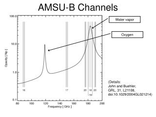
AMSU-B Channels. Water vapor. Oxygen. (Details: John and Buehler, GRL, 31, L21108, doi:10.1029/2004GL021214). AMSU-B Channels. Water vapor. Oxygen. (Figure by Viju O. John). AMSU-B Jacobians. 20 19 18 19 20. ARTS Simulation, Atmosphere: Midlatitude-Summer. (Figure by Viju O. John).

AMSU-B Channels
E N D
Presentation Transcript
AMSU-B Channels Water vapor Oxygen (Details:John and Buehler,GRL, 31, L21108, doi:10.1029/2004GL021214)
AMSU-B Channels Water vapor Oxygen (Figure by Viju O. John)
AMSU-B Jacobians 20 19 18 19 20 ARTS Simulation, Atmosphere: Midlatitude-Summer (Figure by Viju O. John)
Jacobians depend on Atmospheric State (Figures by Viju O. John) • Measurement not in TTL, but below • Altitude where OLR is very sensitive to H2O changes
1D-Var RETRIEVALS AND THE COST FUNCTION It can be shown that maximum likelihood approach to solving the inverse problem (which is a particular case of the generalized analysis problem covered in previous lectures replacing T(z) with a vector x and L with y) requires the minimization of acost functionJ which is a combination of 2 distinct terms. 1D state or profile Radiance vector RT equation Fit of the solution to the measured radiances (y) weighted inversely by the measurement error covariance R (observation error + error in observation operator H) Fit of the solution to the background estimate of the atmospheric state weighted inversely by the background error covariance B The solution obtained is optimal in that it fits the prior (or background) information and and measured radiances respecting the uncertainty in both.
Analysis 12-hour forecast Data Assimilation Background Analysis Observations Model variables, e.g. temperature “True” state of the atmosphere 12 UTC 5 May 00 UTC 6 May 12 UTC 6 May 00 UTC 5 May
Improving vertical resolution with hyper-spectral instruments (AIRS / IASI) Many thousands of channels improves things, but the vertical resolution is still limited by the physics
RETAINING USEFUL INFORMATION ABOVE CLOUDS (Cloud detection scheme for AIRS / IASI) A non-linear pattern recognition algorithm is applied to departures of the observed radiance spectra from a computed clear-sky background spectra. This identifies the characteristic signal of cloud in the data and allows contaminated channels to be rejected AIRS channel 226 at 13.5micron (peak about 600hPa) obs-calc (K) Vertically ranked channel index AIRS channel 787 at 11.0 micron (surface sensing window channel) unaffected channels assimilated CLOUD pressure (hPa) contaminated channels rejected temperature jacobian (K)
CONTENUTI INTEGRATI COLONNARI DI GAS: Principi generali: l'assorbimento differenziale • VAPOR D'ACQUA. • O2 come misura della pressione superficiale • OZONO
Thermosphere O3 layer Stratosphere NO Mesosphere 120 p,T O H O N N O O CH HNO 2 3 2 4 3 2 110 100 90 80 70 Altitude [km] 60 50 40 30 20 10 Troposphere 0 MIPAS Near Real Time productsTarget species
MIPAS possible products MIPAS can simultaneously observe most molecular constituents of the Earth’s atmosphere
Complementary ENVISAT measurements Clear colours:operational Shaded colours: further scientific targets GOMOS: Stratosph.MIPAS: upper Troposph. - lower Mesosphere SCIA:Troposph. - lower Mesosph.
SUPERFICIE TEMPERATURA VAPOR D’ACQUA OZONO CH4 CO
Limb emission measurements Limb measurements resolve the vertical structure of the atmosphere and emission measurements provides continuous (global) geographical coverage.
Aerosols • UV based (only absorbing aerosols: dependence from the vertical distribution) • VIS based • IR (only some type of aerosols (volcanic) • Lidar • Limb profiling (upper atmosphere) • Attempt of retrieving aerosol profile from measurements in the O2 A-Band (760 nm) In general aerosols in the atmosphere are represented with 2 parameters optical thickness at a given wavelength (amount) and aerosol model (type).
Ls=Lp+Lr+Lw Lp=F(aerosols,p) Lr=F(observation geometry, wind (foam, roughness, glint)) Aerosols=F(Ls670,Ls870)
Observation geometry Aerosols amount Aerosols type Aerosols type dependent variables Reflectances depends from aerosols amount and type The ratio of reflectances (an estimation of color of the aerosols) is independent from the amount and used to selecte the aerosol type Once the type is selected optical properties (ω,P) from LUT are used to compute τ
lidar Comment: only 1 wavelength
Aerosols • CONTENUTO COLONNARE/SPESSORE OTTICO • TIPO • PROFILO VERTICALE • PROFILI VERTICALI DI TEMPERATURA E DI CONCENTRAZIONE DI GAS. • profilo di temperatura • Profilo verticale di vapor d'acqua • PARAMETRI D'INSTABILITA'
Atmospheric Profile Retrieval from MODIS Radiances ps I = sfc B(T(ps)) (ps) - B(T(p)) [ d(p) / dp ] dp . o I1, I2, I3, .... , In are measured with MODIS P(sfc) and T(sfc) come from ground based conventional observations (p) are calculated with physics models Regression relationship is inferred from (1) global set of in situ radiosonde reports, (2) calculation of expected radiances, and (3) statistical regression of observed raob profiles and calculated MODIS radiances Need RT model, estimate of sfc, and MODIS radiances
MODIS bands 30-36 MODIS bands 20-29
Parametri dinamici • VENTO ORIZZONTALE IN QUOTA: • VENTO ORIZZONTALE ALLA SUPERFICIE DEL MARE: • VELOCITA' VERTICALE: • CORRENTI MARINE SUPERFICIALI: • Oceanografia • SST • Ocean Colour Clorofilla+correzione aerosols • topografia • Bilancio Radiativo • COMPONENTI DEL BILANCIO RADIATIVO • Boundary layer fluxes • Latent heat flux • sensible heat flux
The trace gas analyses reported in this study started from calibrated radiance measurements from GOME channel 2 (311-405 nm), where the spectral sampling is 0.12 nm at a resolution of 0.18 nm (FWHM). Slant column amounts of SO2, OClO, and BrO have been calculated from the measured radiances using the technique of differential optical absorption spectroscopy (DOAS). Given a background spectrum IB( ) and the earth radiance I( ), both measured by GOME, and absorption cross sections i( ) of the relevant species, their slant column densities Li are fitted together with polynomial coefficients cj according to the Lambert-Beer law for the optical density • D = ln [IB( ) / I( )] = Li i( ) + cj j • For each trace gas, the table below summarizes the selected wavelength window and the references included in the fit. • Window [nm]References • 314-327SO2,O3 • 357-381OClO, NO2, O4, Ring • 345-359BrO, O3, NO2, Ring
GOME fit results (blue) for SO2, OClO, and BrO, compared to reference absorption cross sections measured in the laboratory (violet red). The difference between each fit result and the corresponding reference spectrum is the overall fit residual. Each spectrum represents a single selected groundpixel. http://earth.esa.int/workshops/ers97/papers/eisinger/#intro