Download
1 / 10
100 likes | 260 Views
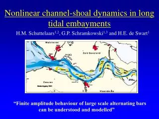
Nonlinear channel-shoal dynamics in long tidal embayments. H.M. Schuttelaars 1,2 , G.P. Schramkowski 1,3 and H.E. de Swart 1. “Finite amplitude behaviour of large scale alternating bars can be understood and modelled”. Observations on large scale alternating bars:.

E N D
Nonlinear channel-shoal dynamics in long tidal embayments H.M. Schuttelaars1,2, G.P. Schramkowski1,3 and H.E. de Swart1 “Finite amplitude behaviour of large scale alternating bars can be understood and modelled”
Observations on large scale alternating bars: • length scales ~ 20 km. • environments with strong tides • fine sand Previous studies: Seminara & Tubino (1998), Hibma et al. (2002) Aim of this talk: to model and understand the observed dynamical behaviour of large scale alternating bars
Model setup • idealised model • straight channel • only bed erodible • depth-averaged SW eqns • suspended load transport • uniform M2 tidal forcing, velocity scale ~ 1 m/s Length scales << channel length, tidal wavelength Typically: • channel width B • horizontal tidal excursion length ~ 7 km
Model approach Use a finite number of spatial patterns obtained from a linear stability analysis to describe the finite amplitude bed behaviour: M N h’ = S SAmn(t) cos (m kcx) cos (npy/B) m=0 n=0 • kc: wavenr. of critical mode • channel length Lc • Lc= ~ 60 km • B ~ 5 km. • N,M: truncation numbers 2p kc kc Growth curves
Model approach 0 0 0 0 Use a finite number of spatial patterns obtained from a linear stability analysis to describe the finite amplitude bed behaviour: M N h’ = S SAmn(t) cos (m kcx) cos (npy/B) m=0 n=0 B m=1,n=1 Lc B m=1,n=2 Lc B m=2,n=1 Growth curves 0 Lc
Model approach Use a finite number of spatial patterns obtained from a linear stability analysis to describe the finite amplitude bed behaviour: M N h’ = S SAmn(t) cos (m kcx) cos (npy/B) m=0 n=0 Insert expansion in complete nonlinear equations. equations describing the behaviour of Amn(t): • steady state solutions • cyclic behaviour
Example: channel width ~ 3.5 km. • multiple steady state solns: • trivial soln. • nontrivial soln. • no steady equilibrium soln for r/sH > 0.0213 periodic soln.
Steady state solution (r~0.0213) Periodic solution (r~0.0214)
Sensitivity study: variation of bed friction and channel width • R<rcr(B): horizontal bed • B<3.6 km: stable static solns. exist • B>3.6 km: no static solns. time-dependency • Small region of multiple stable steady states
Conclusions • existence of finite amplitude alternating bars explicitly • demonstrated • qualitative behaviour depends on channel width and • strength of bed friction • saturation mechanism: importance of destabilizing • sediment fluxes decreases relative to bedslope effects Present work • explore towards realistic values of bed friction • further identification of physical processes • comparison with more complex models