Polynomials
Polynomials. Content. Evaluation Root finding Root Bracketing Interpolation Resultant. Introduction. Best understood and most applied functions Taylor’s expansion Basis of parametric curve/surface Data fitting Basic Theorem: Weierstrass Approximation Theorem


Polynomials
E N D
Presentation Transcript
Content • Evaluation • Root finding • Root Bracketing • Interpolation • Resultant
Introduction • Best understood and most applied functions • Taylor’s expansion • Basis of parametric curve/surface • Data fitting • Basic Theorem: • Weierstrass Approximation Theorem • Fundamental Theorem of Algebra
Compare number of multiplications and additions Evaluate p(t) p(t) = b0 Evaluation – Horner’s Method
Evaluate p(t) and p’(t) p(t) = b0 p’(t) = c1 Details (cont)
Evaluating xk Efficiently • Instead of using pow(x,k), or any iterative/recursive subroutines, think again! • The S-and-X method: S(square) X(multiply-by-x) • See how it works in the next pages • Understand how to implement in program
Each symbol, S or X, represents a multiplication Except for the leading digit, replace 1 by [SX], 0 by [S] • Say the exponent k in base-2: a2a1a0 (k>3) 7 4 3 3 # of :
Right-to-left scan 23 2 1 11 2 1 5 2 2 2 1 1 0 2 0 1 Implementation Left-to-right scan 1 0 1 1 1 z x2 x16 x8 x4 x
[Multiplication, division] • FFT… • GCD of polynomials (Euler algorithm)
Cubics Quadratics Roots of Polynomials • Low order polynomials (for degree 4) Hi-precision formula for quadratics Quartics: see notes
Root Counting • P(x) has n complex roots, counting multiplicities • If ai’s are all real, then the complex roots occur in conjugate pairs. • Descarte’s rules of sign • Sturm’s sequence • Bounds on roots • [Deflation]
Theorems for Polynomial Equations • Sturm theorem: • The number of real roots of an algebraic equation with real coefficients whose real roots are simple over an interval, the endpoints of which are not roots, is equal to the difference between the number of sign changes of the Sturm chains formed for the interval ends.
Sturm Theorem (cont) • For roots with multiplicity: • The theorem does not apply, but … • The new equation : f(x)/gcd(f(x),f’(x)) • All roots are simple • All roots are same as f(x)
A method of determining the maximum number of positive and negative real roots of a polynomial. For positive roots, start with the sign of the coefficient of the lowest power. Count the number of sign changes n as you proceed from the lowest to the highest power (ignoring powers which do not appear). Then n is the maximum number of positive roots. For negative roots, starting with a polynomial f(x), write a new polynomial f(-x) with the signs of all odd powers reversed, while leaving the signs of the even powers unchanged. Then proceed as before to count the number of sign changes n. Then n is the maximum number of negative roots. Descarte’s Sign Rule 3 positive roots 4 negative roots
Computing Roots Numerically • Newton is the main method for root finding • Can be implemented efficiently using Horner’s method • Quadratic convergence except for multiple root • Use deflation to resolve root multiplicity; but can accumulate error; polynomials are sensitive to coefficient variations • Newton-Maehly’s method: roots converges quadratically even if previous roots are inaccurate
Experiment • P(x)=(x-1)(x-2)(x-3)(x2+1) • Assume two imprecise roots have been found, 1.1 & 1.9 • The deflated (cubic) polynomial is then x3-3x2+0.91x-3
Original quintic Converged to 3 in many steps (5 was not a good guess for 3) Deflated cubic Faster convergence, but solution was plagued with the propagated error Maehly procedure Fast convergence; accurate solution
Polynomial Interpolation • Given (n+1) pairs of points (xi,f(xi)) find a nth-degree polynomial Pn(x) to pass through these points • Compute the function value not listed in the table by evaluating the interpolating polynomial
Lagrange Polynomial • High computational cost; cannot reuse points • Divided difference: a better alternative
Resultant (of two polynomials) • An expression involving polynomial coefficients such that the vanishing of the expression is necessary and sufficient for these polynomials to have a common zero.
Resultant (cont) with The above system has common zero: The equation Qz = 0 has nonzero solution IFF R=det(Q) vanishes. R is called the resultant of the equations.
Applications of Resultant II. Algebraic curve intersection I. Common zero III. Implicitization R(x) = 0 IFF intersection exists
Find Common Zero • The system has simultaneous zero iff the resultant is zero
Result from Linear Algebra has non-trivial solution if det(A) = 0 A reduced system (remove row n) gives the ratio: Ai: remove column i
Sylvester Resultant • To find the common zero, consider the reduced system
Resultant in Maxima x as independent variable
Algebraic Curve Intersection No real roots; no intersection (circle & hyperbola)
Algebraic Curve Intersection 2 real roots; 2 intersection points
Implicitization The above system in t has a common zero whenever(x,y) is a point on the curve. … a parabola Application: parametric curve intersection Find the corresponding parameter of (x,y) on the curve
Parametric Curve Intersection implicitize F(s)=f(x(s),y(s))=0 f(x,y)=0 Find roots in [0,1] Bernstein polynomial Cubic Bezier curve and its control points
Quadratic Bezier Curve Intersection Sketch using de Casteljau algorithm [1, 2]
De Casteljau Algorithm [ref] A cubic Bezier curve with 4 control points p(t), t[0,1] is defined. Locate p(0.5)
Given (x,y) on the curve, find the corresponding parameter t Inversion Example