Download
1 / 32
320 likes | 443 Views
Image Processing. Segmentation Process of partitioning a digital image into multiple segments (sets of pixels). 2. Clustering pixels into salient image regions, i.e., regions corresponding to individual surfaces, objects, or natural parts of objects. Image Processing. Segmentation

E N D
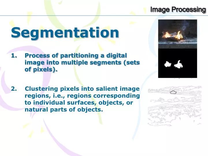
Image Processing Segmentation Process of partitioning a digital image into multiple segments (sets of pixels). 2. Clustering pixels into salient image regions, i.e., regions corresponding to individual surfaces, objects, or natural parts of objects.
Image Processing Segmentation Used to locate objects and boundaries (lines, curves, etc.) in images. Process of assigning a label to every pixel in an image such that pixels with the same label share certain visual characteristics.
Image Processing Segmentation Two of the most common techniques: thresholding and edgefinding
Image Processing Segmentation Two of the most common techniques: edgefinding thresholding
The original image: The objects in image: Three basic types of gray-level discontinuities in a digital image: points, lines. edges. Image Processing B. Detection of discontinuities
run a mask through the image R = f(x-1, y-1) * M1 + f(x, y-1) * M2+ f(x+1, y-1) * M3 + f(x-1, y) * M4 + f(x, y) * M5 + f(x+1, y) * M6 + f(x-1, y+1)* M7+ f(x, y+1)* M8 + f(x+1, y+1)* M9 Image Processing The common way
Image Processing run a mask through the image The common way R = f(x-1, y-1) * M1 + f(x, y-1) * M2+ f(x+1, y-1) * M3 + f(x-1, y) * M4 + f(x, y) * M5 + f(x+1, y) * M6 + f(x-1, y+1)* M7+ f(x, y+1)* M8 + f(x+1, y+1)* M9 Select some threshold . If |R(x,y)| then (x,y) to belong to object (background).
b) a) • Original and segmented images: • Mask H8 • Threshold = 2 • If R(x,y) 2 Then g(x,y) = 1 • Else g(x,y) = 0 H8= Image Processing Example
A masks are usualy used for detection of isolated points in an image are: Image Processing Line detection
Image Processing Example of line detection The original I image and segmented image Io with horizotal mask
Image Processing Example of line detection The original I image and segmented image I45 with 45o mask
Image Processing Example of line detection The original I image and segmented image Iv with vertical mask
Image Processing Example of line detection The original I image and segmented image I135 with 135o mask
Image Processing Example of line detection The original I image and segmented image I8 with H8 mask
Image Processing Formula: Set (x,y): R=0 for k=1 to 3 for q=1 to 3 R = R + f(x+k-2,y+q-2)*M(k,q) If R Then g(x,y) = 255 (object) Else g(x,y) = 0 (non-object) 1 x ImageWidth 1 y ImageHeight
Image Processing Egde detection:
Image Processing Egde detection:
Image Processing Gradient-based procedure:
Image Processing The function f(x) is defined as horizontal gray-level of the image. Gradient-based procedure: The first derivative f’(x) is positive at the point of transition into and out of the ramp as moving from left to right along the profile.
A point M is being an edge point if its two-dimention first order derivative is greater than a specified threshold. Image Processing Gradient-based procedure:
Image Processing If using the second-derivative to define the edge points in an image as the zero crossing of its second derivative. Gradient-based procedure:
Image Processing The signs of second derivative can be used to determine an edge pixel lies on the dark or light side of an edge Gradient-based procedure:
Image Processing The zero crossing property of the second derivative is quite useful for locating the centers of thick edges. Gradient-based procedure:
Image Processing The first is gradient vector of an image f(x, y), and The second is quantity (magnitude) of gradient vector Gradient-based procedure:
Image Processing Gx = (W7 + W8 + W9) – (W1 + W2 + W3) Gy = (W3 + W6 + W9) – (W1 + W4 + W7) The Prewitt gradient vector for detecting x-direction (y-direction) and the Prewitt gradient vectors for detecting diagonal edges: Gx = (W2 + W3 + W6) – (W4 + W7 + W8) Gy = (W6 + W8 + W9) – (W1 + W2 + W4)
Image Processing The general formula for i = 2 to Height-1 for j = 2 to Width-1 { t1 = 0 t2 = 0 for p = 1 to 3 for q = 1 to 3 { t1 = t1 + G1[p, q] * f[i+p-2, j+q-2] t2 = t2 + G2[p, q] * f[i+p-2, j+q-2]} ts = Abs(t1) + Abs(t2) if ts > then Q[i,j] = 1 else Q[i,j] = 0 } }
W Image Processing For the window W from image I, caculating the value R(3,3) = |Dx*W| + |Dy*W| = |-6+12| + |-6+12| = 12 For all pixels of I, except boundary of I, we have matrix R: Example If using threshold at 10:
Image Processing The Prewitt gradient vector for detecting x-direction (y-direction) and the Prewitt gradient vectors for detecting diagonal edges:
Image Processing Gx = (W7 + 2W8 + W9) – (W1 + 2W2 + W3) Gy = (W3 + 2W6 + W9 )– (W1 + 2W4 + W7) The Sobel gradient vector for detecting diagonal edges: The Sobel gradient vector for detecting x-direction and y-direction edges: G1= (W2 + 2W3 + W6 ) – (W4 + 2W7 + W8) G2= (W6 + 2W9 + W8 ) – (W2 + 2W1 + W4)
Image Processing Examples of Sobel filter
Image Processing Second-order derivative: The Laplacian
Image Processing Second-order derivative: The Laplacian The Laplacian is not used in its original form for edge detection (because of sensitive to noise). The Laplacian is combined with smoothing as a precursor to finding edges via zero-crossing.