Download
1 / 16
160 likes | 306 Views
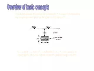
Overview of basic concepts. The background related to problem 7-3 involves two key concepts presented by Berger in Chapter 7. k = 0.001, i = 50 o , F E = 43000nT, z = 1.75m and the equivalent circular cross section yields radius 0.4m. I. F A.

E N D
Overview of basic concepts The background related to problem 7-3 involves two key concepts presented by Berger in Chapter 7. k = 0.001, i = 50o, FE = 43000nT, z = 1.75m and the equivalent circular cross section yields radius 0.4m.
I. FA When FA (the anomalous field) is small, we consider the difference T = FET - FE to be equivalent to the projection of vector FA onto the direction of the main field.
II. FAT is the projection of FA onto the direction of the main field FE, and is considered equal to T, the scalar difference between FE and FET.
Which leads to a basic definition of FAT in terms of HA and ZA, the horizontal and vertical components of the field produced by a buried dipole or sphere.
In the last lecture we derived expressions for HA and ZA assuming vertical inclination. Those equations were good only for that special case. When we consider the influence of arbitrary inclination i, the equations for HA and ZA become more complicated. In problem 7-3 i is 50o so we would have to use equations 7-36 and 7-37 to determine HA and ZA.
What we’re doing here is forward modeling. A question is proposed - “Can the wall be detected?” To answer it we have to calculate the anticipated value of the anomaly that is likely to be observed over this buried wall. You would want to do this before spending lots of time and money running off into the field to collect a big data set only to find that the magnetic field of the wall is too small to observe. Modeling is often a necessary and important preparation for field work.
Short Cut Instead of using equations 7-36 and 7-37, I asked you to use the equations developed for an inclination of 90o … and to solve these two equations at x=0. You were then to compare ZA derived above to the values obtained using equations 7-36 and 7-37 cited in the handout and in the preceding discussion. The above equations for the vertically polarized sphere are easier to evaluate and provide a rough estimate of the anticipated anomaly.
Below are plots of ZA and HA for a range of x. FAT computed for an i of 50o using Berger’s equations yielded a peak anomaly of 6.5nT. Assuming i = 90o we get a Z of ~4.5 nT, which would lead us to the same conclusion - The wall should be detectable.
Let’s see what the computer thinks. extents - 8.1nT 0.27 meter extents 2.1 nT This model does suggest that a sphere does not provide a very good estimate of the anomaly likely to be encountered across a cylinder (or long wall) of equal cross sectional area.
How good are equations 7-36 and 7-37? FAT derived from them yields a maximum anomaly of over 6.5nT. Estimates made assuming vertical polarization yield an anomaly of 4.5 nT and MAGIX suggests that the anomaly over the sphere would be about 2.1nT. We’ve gotten a variety of answers here. Can we sort out the truth? Berger notes that the source of his equations is Telford et al. (Applied Geophysics). Examination of Telford’s text reveals that Berger’s equations are different. Telford’s equations for Z and H are as follows.
Using Telford’s equations we get maximum total anomaly of 3.8nT. This is in much better agreement with the MAGIX model. Can you think of other sources of error that might lead to differences between the model developed in MAGIX and that calculated from Telford’s equations? and It is difficult to accurately portray a sphere in MAGIX using extents in and out. The MAGIX model is not a true 3D representation of the sphere.
We do conclude that the wall will be detectable, but this result is based moreso on the results of MAGIX modeling of a wall with infinite extents rather than from the values obtained approximating the wall by a localized spherical concentration of magnetic material. 2 and 3 NT anomalies are just above the threshold of detection. However, if even small levels of background noise are present such anomalies may be very difficult to spot with confidence.