Linear Algebraic Equations Part 3

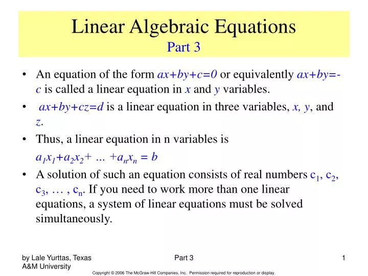
1. Linear Algebraic EquationsPart 3 • An equation of the form ax+by+c=0 or equivalently ax+by=-c is called a linear equation in x and y variables. • ax+by+cz=d is a linear equation in three variables, x, y, and z. • Thus, a linear equation in n variables is a1x1+a2x2+ … +anxn = b • A solution of such an equation consists of real numbers c1, c2, c3, … , cn. If you need to work more than one linear equations, a system of linear equations must be solved simultaneously. Part 3

2. Noncomputer Methods for Solving Systems of Equations • For small number of equations (n ≤ 3) linear equations can be solved readily by simple techniques such as “method of elimination.” • Linear algebra provides the tools to solve such systems of linear equations. • Nowadays, easy access to computers makes the solution of large sets of linear algebraic equations possible and practical. Part 3

3. Gauss EliminationChapter 9 Solving Small Numbers of Equations • There are many ways to solve a system of linear equations: • Graphical method • Cramer’s rule • Method of elimination • Computer methods For n ≤ 3 Part 3

4. Graphical Method • For two equations: • Solve both equations for x2: Part 3

5. Fig. 9.1 • Plot x2 vs. x1 on rectilinear paper, the intersection of the lines present the solution. Part 3

6. Figure 9.2 Part 3

7. Determinants and Cramer’s Rule • Determinant can be illustrated for a set of three equations: • Where [A] is the coefficient matrix: Part 3

8. Assuming all matrices are square matrices, there is a number associated with each square matrix [A] called the determinant, D, of [A]. If [A] is order 1, then [A] has one element: [A]=[a11] D=a11 • For a square matrix of order 3, the minor of an element aij is the determinant of the matrix of order 2 by deleting row i and column j of [A]. Part 3

9. Part 3

10. Cramer’s rule expresses the solution of a systems of linear equations in terms of ratios of determinants of the array of coefficients of the equations. For example, x1 would be computed as: Part 3

11. Method of Elimination • The basic strategy is to successively solve one of the equations of the set for one of the unknowns and to eliminate that variable from the remaining equations by substitution. • The elimination of unknowns can be extended to systems with more than two or three equations; however, the method becomes extremely tedious to solve by hand. Part 3

12. Naive Gauss Elimination • Extension of method of elimination to large sets of equations by developing a systematic scheme or algorithm to eliminate unknowns and to back substitute. • As in the case of the solution of two equations, the technique for n equations consists of two phases: • Forward elimination of unknowns • Back substitution Part 3

13. Fig. 9.3 Part 3

14. Pitfalls of Elimination Methods • Division by zero. It is possible that during both elimination and back-substitution phases a division by zero can occur. • Round-off errors. • Ill-conditioned systems. Systems where small changes in coefficients result in large changes in the solution. Alternatively, it happens when two or more equations are nearly identical, resulting a wide ranges of answers to approximately satisfy the equations. Since round off errors can induce small changes in the coefficients, these changes can lead to large solution errors. Part 3

15. Singular systems. When two equations are identical, we would loose one degree of freedom and be dealing with the impossible case of n-1 equations for n unknowns. For large sets of equations, it may not be obvious however. The fact that the determinant of a singular system is zero can be used and tested by computer algorithm after the elimination stage. If a zero diagonal element is created, calculation is terminated. Part 3

16. Techniques for Improving Solutions • Use of more significant figures. • Pivoting. If a pivot element is zero, normalization step leads to division by zero. The same problem may arise, when the pivot element is close to zero. Problem can be avoided: • Partial pivoting. Switching the rows so that the largest element is the pivot element. • Complete pivoting. Searching for the largest element in all rows and columns then switching. Part 3

17. Gauss-Jordan • It is a variation of Gauss elimination. The major differences are: • When an unknown is eliminated, it is eliminated from all other equations rather than just the subsequent ones. • All rows are normalized by dividing them by their pivot elements. • Elimination step results in an identity matrix. • Consequently, it is not necessary to employ back substitution to obtain solution. Part 3

18. LU Decomposition and Matrix InversionChapter 10 • Provides an efficient way to compute matrix inverse by separating the time consuming elimination of the Matrix [A] from manipulations of the right-hand side {B}. • Gauss elimination, in which the forward elimination comprises the bulk of the computational effort, can be implemented as an LU decomposition. Part 3

19. If L- lower triangular matrix U- upper triangular matrix Then, [A]{X}={B} can be decomposed into two matrices [L] and [U] such that [L][U]=[A] [L][U]{X}={B} Similar to first phase of Gauss elimination, consider [U]{X}={D} [L]{D}={B} • [L]{D}={B} is used to generate an intermediate vector {D} by forward substitution • Then, [U]{X}={D} is used to get {X} by back substitution. Part 3

20. Fig.10.1 Part 3

21. LU decomposition • requires the same total FLOPS as for Gauss elimination. • Saves computing time by separating time-consuming elimination step from the manipulations of the right hand side. • Provides efficient means to compute the matrix inverse Part 3

22. Error Analysis and System Condition • Inverse of a matrix provides a means to test whether systems are ill-conditioned. • Vector and Matrix Norms • Norm is a real-valued function that provides a measure of size or “length” of vectors and matrices. Norms are useful in studying the error behavior of algorithms. Part 3

23. Part 3

24. Figure 10.6 Part 3

25. The length of this vector can be simply computed as Length or Euclidean norm of [F] • For an n dimensional vector Frobenius norm Part 3

26. Frobenius norm provides a single value to quantify the “size” of [A]. Matrix Condition Number • Defined as • For a matrix [A], this number will be greater than or equal to 1. Part 3

27. That is, the relative error of the norm of the computed solution can be as large as the relative error of the norm of the coefficients of [A] multiplied by the condition number. • For example, if the coefficients of [A] are known to t-digit precision (rounding errors~10-t) and Cond [A]=10c, the solution [X] may be valid to only t-c digits (rounding errors~10c-t). Part 3

28. Special Matrices and Gauss-SeidelChapter 11 • Certain matrices have particular structures that can be exploited to develop efficient solution schemes. • A banded matrix is a square matrix that has all elements equal to zero, with the exception of a band centered on the main diagonal. These matrices typically occur in solution of differential equations. • The dimensions of a banded system can be quantified by two parameters: the band width BW and half-bandwidth HBW. These two values are related by BW=2HBW+1. • Gauss elimination or conventional LU decomposition methods are inefficient in solving banded equations because pivoting becomes unnecessary. Part 3

29. Figure 11.1 Part 3

30. Tridiagonal Systems • A tridiagonal system has a bandwidth of 3: • An efficient LU decomposition method, called Thomas algorithm, can be used to solve such an equation. The algorithm consists of three steps: decomposition, forward and back substitution, and has all the advantages of LU decomposition. Part 3

31. Gauss-Seidel • Iterative or approximate methods provide an alternative to the elimination methods. The Gauss-Seidel method is the most commonly used iterative method. • The system [A]{X}={B} is reshaped by solving the first equation for x1, the second equation for x2, and the third for x3, …and nth equation for xn. For conciseness, we will limit ourselves to a 3x3 set of equations. Part 3

32. Now we can start the solution process by choosing guesses for the x’s. A simple way to obtain initial guesses is to assume that they are zero. These zeros can be substituted into x1equation to calculate a new x1=b1/a11. Part 3

33. New x1 is substituted to calculate x2 and x3. The procedure is repeated until the convergence criterion is satisfied: For all i, where j and j-1 are the present and previous iterations. Part 3

34. Fig. 11.4 Part 3

35. Convergence Criterion for Gauss-Seidel Method • The Gauss-Seidel method has two fundamental problems as any iterative method: • It is sometimes nonconvergent, and • If it converges, converges very slowly. • Recalling that sufficient conditions for convergence of two linear equations, u(x,y) and v(x,y) are Part 3

36. Similarly, in case of two simultaneous equations, the Gauss-Seidel algorithm can be expressed as Part 3

37. Substitution into convergence criterion of two linear equations yield: • In other words, the absolute values of the slopes must be less than unity for convergence: Part 3

38. Figure 11.5 Part 3