Download
1 / 6
70 likes | 225 Views
11.5.1 Algebraic Equations. Goto Matlab. roots([1 -4 7 -5]). 1.2151 + 1.3071i 1.2151 - 1.3071i 1.5698. 11.5.2 Succesive Approximation. x=0:0.1:10 y1= tan(x) y2 =5*x plot (x,y1,x,y2) grid axis([0 2 -10 10]) axis([1.3 1.5 6 8]) 1.4.

E N D
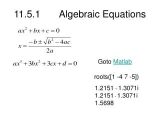
11.5.1 Algebraic Equations Goto Matlab roots([1 -4 7 -5]) 1.2151 + 1.3071i 1.2151 - 1.3071i 1.5698
11.5.2 Succesive Approximation x=0:0.1:10 y1= tan(x) y2 =5*x plot (x,y1,x,y2) grid axis([0 2 -10 10]) axis([1.3 1.5 6 8]) 1.4
11.5.3 Graphical Location of Roots x=0:0.01:3 y1= 15*x.^3+95*x y2 =68*x.^2+47 plot (x,y1,x,y2) Grid At 2.5 z=2.5; diff =1; tol =0.00001; while (diff>tol) z3 = 68/15*z.^2-95/15*z+47/15; zn = z3^(1/3); diff = abs(zn-z); fprintf('%6.4f %6.4f %6.4f \n',z, zn, diff); z=zn; end
x=1.4; diff =1; tol =0.000001; while diff>tol fx= tan(x)-5*x; fdx = (sec(x))^2-5; xn =x-fx/fdx; diff = abs(xn-x); fprintf('%6.4f %6.4f %6.4f \n',x,xn,diff); x=xn; end
11.5.5 Search Method Linear interpolation between to point x=1.4; i=1; fx= fcn(x); while fx <-0.00001 fx =fcn(x); fprintf('%g %6.4f %6.4f \n',i,x,fx); x=x+.0001; i=i+1; end