Precise Digital Leveling
Precise Digital Leveling. Section 4 Geodesy and Corrections for Leveling. Leveled Height Differences. B. Topography. A. C. GRACE Gravity Model 01 - Released July 2003. Image credit: University of Texas Center for Space Research and NASA. Ellipsoid Surface. Geopotential Surfaces.


Precise Digital Leveling
E N D
Presentation Transcript
Precise Digital Leveling Section 4 Geodesy and Corrections for Leveling
Leveled Height Differences B Topography A C
GRACE Gravity Model 01 - Released July 2003 Image credit: University of Texas Center for Space Research and NASA
Ellipsoid Surface Geopotential Surfaces The Geoid Gravity Vector The relationships between the ellipsoid surface (solid red), various geopotential surfaces (dashed blue), and the geoid (solid blue). The geoid exists approximately at mean sea level (MSL). Not shown is the actual surface of the earth, which coincides with MSL but is generally above the geoid.
Level Surfaces and Orthometric Heights Earth’s Surface WP Level Surfaces P Plumb Line Mean Sea Level “Geoid” WO PO Level Surface = Equipotential Surface (W) Ocean Geopotential Number (CP) = WP -WO H (Orthometric Height) = Distance along plumb line (PO to P) Area of Low Density Rock Area of High Density Rock
WGS 84, NAD 83 (86) NAVD 88, NGVD 29 MHHW,MHW, MTL, DTL, MLW, MLLW Tidal Datums Vertical Datum Relationships 3-D Datums Orthometric Datums
SB SF Line of Sight Horizontal CB CF Surface Equipotential Direction of Gravity Curvature Error, C, Where the Line of Sight Is not Parallel to an Equipotential Surface Cancels if SB = SF
Rod B Rod A Shimmer Shorten setup distances – instrument to rod Balance setups – minimize differences Observe over similar surfaces
Crossing a Highway Avoid if Possible Minimize Dissimilar Backsight - Foresight Observing Conditions
Rod 1 Rod 2 Rod 1 F2cos P1 F1cos P2 B2cos P2 B1cos P1 Systematic effect of plumbing error (and scale errors) is small on flat terrain, since B1≈ F2 and F1 ≈ B2
Rod 1 Rod 2 Rod 1 F2cos P1 B2cos P2 F1cos P2 B1cos P1 Systematic effect of plumbing error (and scale errors) accumulates on sloping terrain, since B1≠ F2 and F1 ≠ B2
Rod Scale Correction Cr =De D = observed Δelevationfor the section in meters e = average length excess of the rod pair in mm/m Length excess is determined in rod calibration process
Rod Calibration – Invar to Bottom Reference Plate
Calibration Report SLAC Metrology Laboratory
Laval University (ULAVAL)
Technical University in Munich (TUM)
Stanford Linear Accelerator Center (SLAC)
Stanford Linear Accelerator Center (SLAC) Additional Notes
Critical Distances: It is already well known in the metrology community that digital levels give inaccurate results at certain distances. Therefore the expansion of these distances have to be evaluated to avoid them during the field measurements. As an example, measurements at and around a critical distance of the DNA03 are shown below.
0.5 m Maintain Line of Sight 0.5 m Above Ground Rod Must be ≥ 0.5 m
Rod Temperature Correction Ct = ( tm– ts ) D· CE tm =meanobserved temperatureof Invar strip ts = standardization temperature of Invar strip D = observed Δelevationbetween the bench marks CE = mean coefficient of thermal expansion
Refraction Correction (thermistors) R = -10-5 γ(S/50)2δ·D S = distance(instrument to rod) in meters γ = 70 δ = observed temperature difference between probes at each setup D = Δelevationfor the setup in units of half-cm
Refraction Error, r, Does Not Cancel on Sloping Terrain Since rB≠ rF, even if SB = SF Cool rF rB Warm SB SF
Rigid Leg Tripod With Thermister Equipment
Refraction Correction (predicted) R = -10-5 γ{S/[(2n)(50)}2 δ · d·W S = distance(instrument to rod) in meters γ = 70 n = number of setups δ = “predicted” temp. diff. d = Δelevationfor the setup in units of half-cm W = weather factorbased upon “sun code” where it equals 0.5 for totally overcast, 1.0 for 50% cloudy, 1.5 for 100% sunny Correction not used when thermistors are used!
Time Zones U.S. NAVY TIME ZONE DESIGNATIONS STANDARD DAYLIGHT TIME TIME ZONE U.S.NAVY TIME TIME MERIDIAN DESCRIP’N DESIGNATION Atlantic AST Eastern EDT 60W +4Q (Quebec) Eastern EST Central CDT 75W +5 R (Romeo) Central CST Mountain MDT 90W +6 S (Sierra) Mountain MST Pacific PDT 105W +7 T (Tango) Pacific PST Yukon YDT 120W +8 U (Uniform) Yukon YST AK/HI HDT 135W +9 V (Victor) AK/HI HST Bering BDT 150W +10 W (Whiskey)
Astronomic Correction Ca =0.7 ·Ks s = section length K = tan εmcos(Am – α) + tan εscos(As – α) where Am = azimuth of the moon; εm = deflection due to the moon; As =azimuth of the sun; εs= deflection due to the sun; α = azimuthof section (Δλ/Δθof adjacent BMs) 0.7 because the earth is elastic
One of Several Corrections Applied to Precise Leveling Leveling Route є a S Reference Surface Maximum Tide N Equilibrium S Effect, a, of tidal deflection, є, on a section of length and direction S
Level Collimation Correction Cc = - (e·SDS) e= collimation error in radians x 1000 or mm/m SDS = accumulated difference in sight lengthsfor the section in meters
Effect of Collimation Error, α Line of Sight S(tan α) α Horizontal S Direction of Gravity
Consistent Collimation Error Cancels In Balanced Setup Since SB = SF α α SB SF Direction of Gravity
Orthometric Correction Co=-2hα·sin2ρ[1+(α–2β/α)cos2ρ]dρ h = average heightof section α = 0.002644; β = 0.000007 ρ = average latitudeof the section dρ = latitudedifferencebetween the beginning and end points of the section Correction not needed when geopotential numbers are used!
All HeightsBasedonGeopotentialNumber (CP) The geopotential number is the potential energy difference between two points g = local gravity; WO = potential at datum (geoid); WP = potential at point • Why use Geopotential Number? - because if the GPN for two points are equal they are at the same potential and water will not flow between them
Geopotential Number O = one point on the geoid A = another point on the geoid connected to “O” by precise leveling dn =Δelevationbetween the Bench Marks g = average value of actual gravity between successive Bench Marks, but to look up g we need θandλ, and we need to know the number of setupssince we are integrating
Geopotential to Orthometric H = C/(g + 0.0424 H0) C = the estimated geopotential number in gpu g = the gravity value at the benchmark in gals H = the orthometric height in kilometers
HeightsBasedonGeopotentialNumber (C) • NormalHeight (NGVD 29) H* = C / • = Average normal gravity along plumb line • DynamicHeight (IGLD 55, 85) Hdyn= C / 45 • 45 = Normal gravity at 45° latitude • OrthometricHeight H = C / g • g = Average gravity along the plumb line • HelmertHeight (NAVD 88) H = C / (g + 0.0424 H0) • g = Surface gravity measurement (mgals)
Idiosyncrasies & Caveats • θ and λ observables are stored in description file • What happens to observations when you create a TBM? • The gravity file is in the NAD27 datum • Temperatures are taken at many places and times • Thermistor probes at each instrument setup • Thermometers at each bench mark • Thermometers on each rod • Wind and sun codes are a very important fallback
Idiosyncrasies & Caveats (Continued) • Tables of constants are tabulated in time and position so time, time zone, and datum are very important • When data are loaded to the data base they are supposed to be statistically free of biases and blunders. • Field specifications and procedures are designed to trap biases and blunders in the field
“Phase 1” Data Office Abstract
Setup of Leveling, Δh = B – F and S = SB + SF Rod 1 Rod 2 Foresight Backsight F B Δh SB SF S