Download
1 / 20
210 likes | 507 Views
Optimization : The min and max of a function. Michael Sedivy Daniel Eiland. Introduction. Given a function F(x), how do we determine the location of a local extreme (min or max value)? Two standard methods exist :. F(x) with global minimum D and local minima B and F.

E N D
Optimization :The min and max of a function Michael Sedivy Daniel Eiland
Introduction Given a function F(x), how do we determine the location of a local extreme (min or max value)? Two standard methods exist : F(x) with global minimum D and local minima B and F Searching methods – Which find local extremes using several sets of values (Points) for each function variable then select the most extreme. Iterative methods – Which select a single starting value (Point) and take “steps” away from it until the same Point is returned
Algorithm Selection Calculation of an extreme is not a perfect thing and is highly dependant upon the input function and available constraints. For basic one-dimensional functions [F(x)] choices include : • Brent’s method – For calculation with or without the derivative • Golden Section Search – For functions with multiple values for a given point
Multi-Dimensional Selection For multi-dimensional, there are two sets of methods which can be grouped by the use (or lack there-of) of the gradient. The gradient is the set of first partial derivatives for a function f and is represented as : For a given point in f, the gradient represents the direction of greatest increase. Gradient of f(x,y) = -(cos2x +cos2y)2 shown below the plane as a vector field
Multi-Dimensional Methods Gradient Independent Methods : • Downhill Simplex Method – “Slow but sure”. A general purpose algorithm that requires O(N2) of storage • Direction Set Method (Powell’s Method) – Much faster than the Downhill method but requires a smooth function Gradient Dependent Methods : • Conjugate Gradient Method – The gradient of the function must be known but only requires O(~3N) storage • Quasi-Newton (or variable metric) methods – Requires O(N2) storage but calculates the gradient automatically
Line Minimization The first step for many one-dimensional and multi-dimensional methods is to determine the general location of the minimum. This based on ability to bracket a minimum between a triplet of points [a,b,c] such that f(a) > f(b) and f(c) > f(b).
Bracketing Calculation of this bracket is straightforward assuming points a and b are supplied. Simply scale the value of b such that is moves further away from a until a point c is found such that f(c) > f(b).
Line Minimization (Con’t) Once c is calculated, the final search for a minimum can be begin. The simplest method (Golden Section Search) is to evaluate a point d, halfway between b & c. If f(d) > f(b), then set c to d otherwise set b to d and a to b. This then process then repeats alternating between the a-b line segment and b-c line segment until the points converge (f(a) == f(b) == f(c)).
Line Minimization (Golden Section) f(d) > f(b) d > b f(d) < f(b) b > d
Brent’s Method While the Golden Section Search is suitable for any function, it can be slow converge. When a given function is smooth, it is possible to use a parabola fitted through the points [a,b,c] to find the minimum in far fewer steps. Known as Brent’s method, it sets point d to the minimum of the parabola derived from :
Brent’s Con’t It then resets the initial points [a,b,c] based on the value of f(d) similar to Golden Section Search. f(d) < f(b) b > d Of course, there is still the matter of the initial points a and b before any method can be applied…
Downhill Simplex Method • Multi-dimensional algorithm that does not use one-dimensional algorithm • Not efficient in terms of function evaluations needed. • Simplex – geometric shape consisting of N+1 vertices, where N= # of dimensions • 2 Dimensions – triangle • 3 Dimensions - tetrahedron
Downhill Simplex Method, cont’d. • Start with N+1 points • With initial point P0, calculate other N points using Pi = P0 + deltaei • Ei – N unit vectors, delta – constant (estimate of problem’s length scale) • Move point where f is largest through opposite face of simplex • Can either be a reflection, expansion, or contraction • Contraction can be done on one dimension or all dimensions • Termination is determined when distance moved after a cycle of steps is smaller than a tolerance • Good idea to restart using P0 as on of the minimum points found. • http://optlab-server.sce.carleton.ca/POAnimations2007/NonLinear7.html
Direction Set/Powell’s Method • Basic Method - Alternates Directions while finding minimums • Inefficient for functions where 2nd derivative is larger in magnitude than other 2nd derivatives. • Need to find alternative for choosing direction
Conjugate Directions • Non-interfering directions (gradient perpendicular to some direction u at the line minimum) • N-line minimizations • Any function can be approximated by the Taylor Series: • Where:
Quadratically Convergent Method • Powell’s procedure – can exactly minimize quadratic form • Can have directions become linearly dependent (finds minimum over subset of f) • Three ways to fix problem: • Re-initialize direction set to basis vectors after N or N+1 iterations of basic procedure • Reset set of directions to columns of any orthogonal matrix • Drop quadratic convergence in favor of finding a few good directions along narrow valleys
Dropping Quadratic Convergence • Still take Pn-P0 as a new direction • Drop old direction of the function’s largest decrease • Best chance to avoid buildup of linear dependence. • Exceptions: • If fE >= 0, avg. direction PN-P0 is done • If 2(f0 – 2fN + fE)[(f0 – fN) - Δf]2 >= (f0 – fE)2 Δf • Decrease along avg. direction not due to single direction’s decrease • Substantial 2nd derivative along avg. direction and near bottom of its minimum
Conjugate Gradient Method Like other iterative methods, the Conjugate Gradient method starts at a given point and “steps” away until it reaches a local minima [maxima can be found by substituting f(x) with –f(x)]. Iterative step-wise calculation of a minima
Calculating the Conjugate Gradient As the name implies, the “step” is based on the direction of the Conjugate Gradient which is defined as : Where h0 = g0and giis the steepest gradient a given point : And yi is a scalar based on the gradient :
Basic Algorithm Given the function f, its gradient and an initial starting point P0. Determine the initial gradient and conjugate values : Iteratively repeat : • Calculate Pi using a line minimization method with the initial points as a=Pi-1 and b=hi • If Pi equals Pi-1; stop • Calculate the new gradient : • Calculate the new conjugate : While this can terminate in O(N) [N = # terms in f] iterations, it is not guaranteed but can still result in fewer computations than the number needed for the Direction Set Method