Download

1 / 14
140 likes | 390 Views
Chapter 7: Matrices and Systems of Equations and Inequalities. 7.1 Systems of Equations 7.2 Solution of Linear Systems in Three Variables 7.3 Solution of Linear Systems by Row Transformations 7.4 Matrix Properties and Operations 7.5 Determinants and Cramer’s Rule

E N D
Chapter 7: Matrices and Systems of Equations and Inequalities 7.1 Systems of Equations 7.2 Solution of Linear Systems in Three Variables 7.3 Solution of Linear Systems by Row Transformations 7.4 Matrix Properties and Operations 7.5 Determinants and Cramer’s Rule 7.6 Solution of Linear Systems by Matrix Inverses 7.7 Systems of Inequalities and Linear Programming 7.8 Partial Fractions
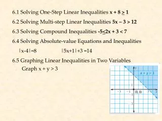
7.7 Systems of Inequalities and Linear Programming • Many mathematical descriptions of real situations are best described as inequalities rather than equations. Some examples: • Using a machine no more than 12 hours a day • Producing at least 500 cases of a certain product to meet a contract • A line divides a plane into three sets of points: • Points on line r, • Points in half-plane P, and • Points in half-plane Q.
7.7 Solving Linear Inequalities • A linear inequality in two variables can take the form where A, B,and C are real numbers. The inequality symbol can be replaced with , <, or >. • The graph of a linear inequality is a half-plane.
7.7 Solving Linear Inequalities Example Graph Solution The boundary line is Since the points on this line do not satisfy we use a dashed line in the graph. The half-plane is above the boundary line.
7.7 Solving Systems of Inequalities Example Graph the solution set of the system. Graphing Calculator Solution Solve each equation for y. Then let
7.7 Solving Systems of Inequalities Analytic Solution Graph the boundary equations x = 6 – 2y and x2 = 2y and find the boundary points (the points of intersection) using the methods from §7.1.
7.7 Linear Programming • An important application of mathematics to business and social science is linear programming. • Linear programming is used to find an optimum value. - minimum cost - maximum profit • First developed to solve problems in allocating supplies for the U.S.Air Force during WWII.
7.7 Linear Programming Example The Charlson Company makes two products: VCRs and DVD players. Each VCR gives a profit of $30, while each DVD player produces a $70 profit. The company must manufacture at least 10 VCRs per day to satisfy one of its customers, but no more than 50 because of production problems. The number of DVD players produced cannot exceed 60 per day, and the number of VCRs cannot exceed the number of DVD players. How many of each should the company manufacture to obtain maximum profit? Let x = number of VCRs to be produced daily, and y = number of DVD players to be produced daily.
7.7 Linear Programming Example At least 10 VCRs must be produced, but no more than 50, so x 10 and x 50. No more than 60 DVD players may be made in one day, so y 60. Number of VCRs may not exceed the number of DVD players: x y. The number of VCRs and DVD players cannot be negative, so x 0 and y 0. These restrictions, or constraints, form the system of inequalities: x 10, x 50, y 60, x y, x 0, y 0.
profit = 30x + 70y 0 = 30x + 70y 1000 = 30x + 70y 3000 = 30x + 70y 7000 = 30x + 70y 7.7 Linear Programming Example To find the maximum possible profit, sketch the graph of each constraint. Find the intersection of the feasible values of x and y; they must satisfy all constraints. Then maximize the objective function: profit = 30x + 70y. Figure 71 pg 7-291 Figure 72 pg 7-292 Figure 73 pg 7-292 The coordinates (50, 60) on the line 5700 = 30x + 70y give a maximum profit. This area is called the region of feasible solutions.
7.7 Fundamental Theorem of Linear Programming Fundamental Theorem of Linear Programming The optimum value for a linear programming problem occurs at a vertex of the region of feasible solutions. • Solving a Linear Programming Problem • Write the objective function and all necessary constraints. • Graph the feasible region. • Identify all vertices or corner points. • Find the value of the objective function at each vertex. • The solution is given by the vertex producing the optimum value of the objective function.
7.7 Finding Minimum Cost Robin takes vitamin pills each day. She wants at least 16 units of Vitamin A, at least 5 units of Vitamin B1, and at least 20 units of Vitamin C. She can choose between red pills, costing 10¢ each, that contain 8 units of A, 1 of B1, and 2 of C; and blue pills, costing 20¢ each, that contain 2 units of A, 1 of B1, and 7 of C. How many of each pill should she buy to minimize her cost and yet fulfill her daily requirements? Solution Let x = number of red pills to buy, and y = number of blue pills to buy. The objective function: cost = 10x + 20y pennies per day
7.7 Finding Minimum Cost At least 16 units of A, 8 from red, 2 from blue. Restrictions: At least 5 units of B1, 1 from red and 1 from blue. At least 20 units of C, 2 from red, 7 from blue. The number of each type of pill cannot be negative. Robin’s best bet is to buy 3 red pills and 2 blue ones for a cost of 70¢ per day.