Download
1 / 18
180 likes | 299 Views
Explore the essentials of Computational Fluid Dynamics (CFD) with a focus on gridding techniques and time-dependent modeling. Under the guidance of Professor William J. Easson at the University of Edinburgh, you will learn how to create geometries in Star-Design, produce various meshes, and solve for laminar flows in 2D channels and jets. Gain insights into structured and unstructured grids, their advantages and disadvantages, and conduct simulations for steady and turbulent flows. Enhance your understanding of time-dependent equations for improved convergence in flow solutions.

E N D
Computational Fluid Dynamics 5Gridding & time-dependance Professor William J Easson School of Engineering and Electronics The University of Edinburgh
Things you can do • Create simple geometries in Star-Design • Produce meshes of different densities and of varying density (by changing the parameters before meshing) • Solve for laminar flow in a 2D channel • Present the output in a variety of formats • Solve for 2D laminar jets • Solve for 2D flows with wall attachment • Solve to 1st & 2nd order simulations (check this) • Test the appropriateness of your mesh density (check) • Test the appropriateness of the extent of your domain
Things you can do • Simulate steady, turbulent flow • Simulate flow past objects in a domain • Calculate the drag coefficient using the sum of forces on an object in a flow • Determine whether flow solution is dominated by hyperbolic, parabolic or elliptic behaviour • Utilise time-dependant equations to enhance convergence for elliptically-dominated solutions
Gridding Anderson and Versteek & Malalasekera both weak on gridding
Structured grids (eg hex) Advantages: • Equations relatively simple • Cell shape is easily controlled • Numerical errors are smaller • Can be fitted to flow direction • Can be fitted to gradients in flow • Optimises memory use Disadvantages: • Fitting to complex geometries requires a lot of time and skill
Un-structured grids (eg tet) Advantages: • Can be fitted to unusual shapes • ‘One-click’ creation Disadvantages: • Generally larger errors • Limited control over cell shape – ‘skewness’
Exercise 1 Simulate laminar flow through a straight pipe 8mm dia and 50mm long. Increase the cell density next to the wall • Using a structured grid by creating a prism layer • Using a triangular grid with a growth function Note the number of cells created in each case and the relative convergence time
Time-dependant flows Anderson Ch4 Versteeg & Malalasekera Ch8
Time dependant modelling • Many flows are inherently time-dependant and therefore require to be modelled as such • Some steady-state flow solutions are not well-behaved and therefore require to be modelled by time-dependent equations to achieve convergence
Classification of NS • General NS equations are of ‘mixed’ class
Explicit techniques • Solution at time-step t+Δt is obtained by marching forward from time-step t and obtaining gradients for estimating new values from those at previous time-step • Easy to program and quick to solve, but can be unstable if Δt too large (conditionally stable) • Δtmax is proportional to (Δx)2, so quickly becomes very small and limits usefulness of solution
Implicit techniques • Solution at time-step t+Δt is obtained by marching forward from time-step t and obtaining gradients for estimating new values from those at previous and current time-step • Crank-Nicolson is an early example • Requires solution of large number of simultaneous equations (also extra ‘loops’ inside iteration process) • Conditionally, or even unconditionally, stable • Large Δt results in errors – not instability • May be quicker to converge than explicit due to improved stability
Time-dependant example Vortex shedding past a cylinder • 2D example • Use laminar flow, 16mm cylinder at 7.5mm/s (Re~120 ) • Create unstructured grid using sizing function • Use an unsteady solver • Calculate the shedding frequency and check that it matches the strouhal number