Download

1 / 13
130 likes | 189 Views
Explore advanced packet classification techniques using coarse-grained tuple spaces, improving lookup efficiency and performance.

E N D
Packet Classification Using Coarse-Grained Tuple Spaces Haoyu Song, Jon Turner and Sarang Dharmapurikar www.arl.wustl.edu
Overview • Two-dimensional packet classification problem • in list of 2d filters, find first match for given address pair • (1011,0111): [<101*,10*>, <10*,011*>, <1*,01*>] • Limitations of current solutions • fast algorithmic methods require excessive space (≥50x) • TCAM has high cost per bit, significant power usage • Combining cross-product and tuple-space search • hybrid strategy with range of time-space tradeoff options • Improving 1d lookups • combining tree bitmap and Bloom filters • Possible extensions
filter set F0: <1010*, 01*>F1: < 101*,0111*> cross product table key filter S0D0F0S0D1F0S1D0noneS1D1F1 Cross-Product Method • Procedure • do 1d lookup on all fields • combine results into lookup key in cross-product table • direct lookup table or hash table • Fast, but space grows as nk for n filters, k fields 10100, 01110 S0D1
0 32 0 Destination IP Prefix Length 32 Source IP Prefix Length 2D Tuple Space Search • Group by prefix length • hash table per group • up to 33 x 33= 1,089 groups • in practice 30-100 occupied tuples • Rectangle search • markers to guide search • at most 33 probes, often less • hard to update • Pruned tuple space search • 1d search on src/dest fields • find prefix lengths that match src/dest fields of packet • search intersecting tuples • if ≤k matching prefixes, at most k2 probes
32 0 0 Destination IP Prefix Length 32 Source IP Prefix Length Coarse-Grained Tuple Space • Select coarse-grained partition of tuple space • Build cross-product table per sub-space • Search procedure • 1d lookups for LPM • probe each subspace • terminate early if possible • Pruning • identify candidate sub-spaces during 1d lookup • probe selected sub-spaces • Space/time tradeoff
Performance of Basic Algorithm • Equal size divisions of 2d tuple space • Ratio of cross-products to filter set size • 2x2 partition brings space usage to 2x minimum • maximum of four probes required • compared to 30-90 for simple tuple space search • Pruning of limited use for filter sets of size <104
4x 3x 2x Performance of Best Configurations
32 0 0 Destination IP Prefix Length 32 Source IP Prefix Length Alternate Partitioning Approaches • Arbitrary sub-spaces are possible • potential for fewer regions with good space efficiency • Preliminary results mixed • may be useful for smaller filter sets • More evaluation needed Note: filters of form <prefix,*> and <*,prefix> stored in 1d data structures
110 1011 1 0 BloomFilters off-chiphash tables 0 0 1 1 0 101 1 0,1 0 1 0 1 0 1 10110 110,111,000,001 3 0 1 1 0 1 10110 10100,10101,10110,10111 0 1 5 Fast 1d Lookups Tree Bitmap Hashing + Bloom Filters • Multibit trie • Co-located children • Bitmaps for • prefix nodes • subtree presence • 4 bit stride implies 8 memory accesses • Expand prefixes to “standard” lengths • Off-chip hash table per length • On-chip Bloom filters to avoid unproductive probes • Large space requirements for good worst-case performance
Bloomfilters subtreehash tables 1 0 0 0 1 1 0 0 1 0 1 1010 2 1 0 1 0 1 1101 4 Fast and Compact 1d Lookups • Insert tree bitmap subtree roots into off-chip hash tables and on-chip Bloom filters • Lookup prefix of subtree roots in Bloom filters • if match on length kand all shorter lengths, probe off-chip table for length k • Reduction in on-chip memory for Bloom filters • shape-shifting trie yields further space reduction
1d Lookup Performance 200K IPv4 prefixes 5 bit stride for tree bitmap 8 bit on-chip “root table” 4 Bloom filters 1 BF entry for every 2 prefixes 1 off-chip probes (4 incl. FP) 2 Bloom filters 1 BF entry for every 6 prefixes 2 off-chip probes (4 incl. FP)
Practical Configuration • Configure 1d lookups for 1 off-chip probe each (excluding false positives) • about 5 bits per prefix for Bloom filters with low FP rate • Record <prefix,*> and <*,prefix> filters in 1d lookup data structures • also proposed in recent paper by Kounavis, et. al. • Divide remaining filters among four subspaces • approximately 2 off-chip hash table entries per filter • at most four probes • With single QDR SRAM at 200 MHz, 32 bit word size can do 200 million probes per second • about 33 million packets/second • 40 byte packets at 10 Gb/s
Possible Extensions • More extensive evaluation • scaling to larger filter sets – 100-200K filters • integrated evaluation of 1d and 2d lookups • systematic evaluation of alternate partitioning strategies • Alternate representations of filter sub-spaces • any filter set data structure is candidate • using decision trees, can skip 1d lookups • Generalization to more dimensions • handling fields with ranges (for port numbers) • coarse-grained grouping of tuple-spaces defined on “nesting level” • can we beat TCAM?