Parallel Visualization At TACC
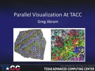
Parallel Visualization At TACC. Greg Abram. Visualization Problems. Huge problems: Data cannot be moved off system where it is computed Visualization requires equivalent resources as source HPC system. Large problems: Data are impractical to move over WAN, costly to move over LAN

Parallel Visualization At TACC
E N D
Presentation Transcript
Parallel Visualization At TACC Greg Abram
Visualization Problems • Huge problems: • Data cannot be moved off system where it is computed • Visualization requires equivalent resources as source HPC system • Large problems: • Data are impractical to move over WAN, costly to move over LAN • Visualization requires parallel systems for enough memory, CPU and GPU • Medium problems: • Data are costly to move over WAN • Visualization requires lots of memory, fast CPU and GPU • Small problems: • Data are small and easily moved • Office machines and laptops are adequate for visualization *With thanks to Sean Ahern for the metaphor
Visualization Problems • Huge problems • Don’t move the data; in-situ and co-processing visualization minimizes or eliminates data I/O • Large problems • Move your data to visualization server and visualize using parallel high-performance systems and software at TACC • Medium and small problems • Move your data to visualization server and visualize using high-performance systems at TACC *With thanks to Sean Ahern for the metaphor
Visualization Servers: Longhorn • 256 compute nodes: • 16 “Fat” nodes - • 8 Intel Nehalem cores • 144 GB • 2 NVIDIA Quadro FX5800 GPUs • 240 standard nodes • 8 Intel Nehalem cores • 48 GB • 2 NVIDIA Quadro FX5800 GPUs • Access (see Longhorn User Guide): • Longhorn Portal, or • Run qsubjob.vnc on Longhorn using normal, development, long, largemem, request queues
Longhorn Architecture largemem request login1.longhorn (longhorn) “Fat” nodes 144 GB RAM 2 GPUs Vis Nodes 48 GB RAM 2 GPUs $HOME normal development long request Longhorn File Systems $SCRATCH Longhorn Visualization Portal /ranger/share normal Queues Retired /ranger/work Login Nodes Compute Nodes /ranger/scratch Read-Only File System Access Read/Write File System Access Job submission Lustre Parallel File System NFS File System Ranger File Systems
Visualization Servers: Stampede • Access to Stampede file systems • 128 Vis nodes: • 16 Intel Sandy Bridge cores • 32 GB RAM • 1 Nvidia K20 GPU • 16 Large Memory Nodes • 32 Intel Sandy Bridge cores • 1 TB RAM • 2 Nvidia K20 GPU • Access (see Stampede User Guide): Run sbatchjob.vnc on Longhorn using vis, largememqueues
Stampede Architecture largemem SHARE normal, serial, development, request 4x login nodes stampede.tacc.utexas.edu WORK Login Nodes SCRATCH 16 LargeMem Nodes 1TB RAM 32 cores 2x NvidiaK20 GPU ~6300 Compute Nodes 32 GB RAM 16 cores Xeon Phi 128 Vis Nodes 32 GB RAM 16 cores Nvidia K20 GPU vis, gpu Queues Stampede Lustre File Systems Compute Nodes Read/Write File System Access Job submission
Parallel Visualization Software • Good news! Paraview and Visit both run in parallel on and look just the same! • Client/Server Architecture • Allocate multiple nodes for vncserver job • Run client process serially on root node • Run server processes on all nodes under MPI
Interactive Remote Desktop system login node Port forwarding Internet VNC viewer … Remote System … VNC server System Vis Nodes
Remote Serial Visualization Visualization GUI System login node Port forwarding Internet … Remote System … visualization process System Vis Nodes
Remote Parallel Visualization Visualization GUI System login node Port forwarding Internet MPI Process … Remote System … Visualization client process Allocated node set Parallel visualization server process System Vis Nodes
Parallel Session Settings • Number of nodes M • more nodes gives you: • More total memory • More I/O bandwidth (up to a limit determined by file system and other system load) • More CPU cores, GPUs (though also affected by wayness) • WaynessN • processes to run on each node • Paraview and Visit are not multi-threaded • N < k gives each process more memory, uses fewer CPU cores for k = number of cores per node • Need N > 1 on Longhorn, Stampede large memory nodes to utilize both GPUs • Longhorn portal: • Number of Nodes and Waynesspulldowns • qsub-peNwayM argument • Mspecifies number of nodes (actually, specify k*M) • N specifies wayness • sbatch –N [#nodes] –n [#processes/node]
Running Paraview In Parallel • Run Paraview as before • In a separate text window: module load python paraview NO_HOSTSORT=1 ibruntacc_xrunpvserver • In Paraview GUI: • File->Connect to bring up the Choose Server dialog • Set the server configuration name to manual • Click Configure and, from Startup Type, select Manual and Save • In Choose Server dialog, select manualand click Connect In client xterm, you should see Waiting for server… and in the server xterm, you should see Client connected.
Running Visit In Parallel • Run Visit as before; it’ll do the right thing
Data-Parallel Visualization Algorithms • Spatially partitioned data are distributed to participating processes…
Data-Parallel Algorithms • Sometimes work well… • Iso-contours • Surfaces can be computed in each partition concurrently and (with ghost zones) independently • However, since surfaces may not be evenly distributed across partitions, may lead to poor load balancing
Data-Parallel Algorithms • Sometimes not so much… • Streamlines are computed incrementally P0 P1 P2 P3
Parallel Rendering • Collect-and-render • Gather all geometry on 1 node and render • Render-and-composite • Render locally, do depth-aware composite • Both PV and Visit have both, offer user control of which to use
Parallel Data Formats • To run in parallel, data must be distributed among parallel subprocess’ memory space • Serial formats are “data-soup” • Data must be read, partitioned and distributed • Parallel formats contain information enabling each subprocess to import its own subset of data simultanously • Maximize bandwith into parallel visualization process • Minimize reshuffling for ghost-zones • Network file system enables any node to access any file
Paraview XML Parallel Formats • Partition data reside in separate files: • .vti regular grids, .vtsfor structured grids … • Example: One of 256 partitions of a 20403 volume: c-2_5_5.vti <?xml version="1.0"?> <VTKFile type="ImageData" version="0.1" byte_order="LittleEndian"> <ImageDataWholeExtent="510 765 1275 1530 1275 1530" Origin="0 0 0" Spacing="1 1 1"> <Piece Extent="510 765 1275 1530 1275 1530"> <PointData Scalars="Scalars_"> <DataArray type="Float32" Name="Scalars_" format="binary" RangeMin="0.0067922524177" RangeMax="1.7320507765"> ….. Encoded data looking lijkeascii gibberish </DataArray> … • Global file associates partitions into overall grid • .pvtiregular grids, .pvtsfor structured grids … • Example: global file for 20403 volume: c.pvti <?xml version="1.0"?> <VTKFile type="PImageData" version="0.1" byte_order="LittleEndian" compressor="vtkZLibDataCompressor"> <PImageDataWholeExtent="0 2040 0 2040 0 2040" GhostLevel="0" Origin="0 0 0" Spacing="1.0 1.0 1.0"> <PPointData Scalars="Scalars_"> <PDataArray type="Float32" Name="Scalars_"/> </PPointData> <Piece Extent="0 255 0 255 0 255" Source="c-0_0_0.vti"/> <Piece Extent="0 255 0 255 255 510" Source="c-0_0_1.vti"/> … <Piece Extent="510 765 1275 1530 1275 1530" Source="c-2_5_5.vti"/> …
SILO Parallel Format • “Native” VisIt format • Not currently supported by Paraview • Built on top of lower-level storage libraries • NetCDF, HDF5, PDB • Multiple partitions in single file simplifies data management • Directory-like structure • Parallel file system enables simultaneous read access to file by multiple nodes • Optimal performance may be a mix • note that write access to silo files is serial
Xdmf Parallel Format • Common parallel format • Seen problems in VisIt • Also built on top of lower-level storage libraries • NetCDF, HDF5 • Multiple partitions in single file simplifies data management • Also directory-like structure • Also leverages Parallel File System • Also optimal performance may be a mix
Data Location • Data must reside on accessible file system • Movement within TACC faster than across Internet, but can still take a long time to transfer between systems Ranch Lonestar Stampede TACC LAN Stampede Lustre PFSs LonestarLustrePFSs Ranger Spur Longhorn Retired Ranger Lustre PFS Longhorn LustrePFS Internet
Post-Processing • Simulation writes periodic timesteps to storage • Visualization loads timestep data from storage, runs visualization algorithms and interacts with user Sim host Storage Viz host … … … …
Postprocessing On HPC Systems and Longhorn Lonestar /Stampede Longhorn Lustre PFS … System Lustre PFS … … … Longhorn
Postprocessing On Stampede 2. Data is read back into vis nodes for visualization 1. Simulation runs on compute nodes, writes data to Lustre file system Stampede … … Lustre PFS
Huge Data: Co- and In-Situ Processing • Visualization requires equivalent horsepower • Not all visualization computation is accelerated • Increasingly, HPC platforms include acceleration • I/O is expensive: simulation to disk, disk to disk, disk to visualization • I/O is not scaling with compute • Data is not always written at full spatial, temporal resolution
Huge Data: Co- and In-Situ Processing • Visualization requires equivalent horsepower • Not all visualization computation is accelerated • Increasingly, HPC platforms include acceleration • I/O is expensive: simulation to disk, disk to disk, disk to visualization • I/O is not scaling with compute • Data is not always written at full spatial, temporal resolution
Co-Processing • Perform simulation and visualization on same host • Concurrently • Communication: • Many-to-many • Using high-performance interconnect to communicate … …
In-Situ Processing • Incorporate visualization directly into simulation • Run visualization algorithms on simulation’s data • Output only visualization results … …
Co- and In-Situ Processing • Not a panacea • Limits scientist’s exploration of the data • Can’t go back in time • May pay off to re-run the simulation • Impacts simulation • May require source-code modification of simulation • May increase simulation node’s footprint • May affect simulation’s stability • Simulation host may not have graphics accelerators • … but visualizations are often not rendering-limited • … and more and more HPC hosts are including accelerators
Co- and In-Situ Status • Bleedingedge • Coprocessing capabilities in Paraview, VisIt • Did I say bleeding edge? • In-Situ visualization is not simple • We can help
Summary • Parallel visualization is only partly about upping the compute power available, its also about getting sufficient memory and I/O bandwidth. • I/O is a really big issue. Planning how to write your data for parallel access, and placing it where it can be accessed quickly, is critical. • The TACC visualization groups are here to help you!