Lecture 11 Vector Spaces and Singular Value Decomposition
Lecture 11 Vector Spaces and Singular Value Decomposition. Syllabus.

Lecture 11 Vector Spaces and Singular Value Decomposition
E N D
Presentation Transcript
Syllabus Lecture 01 Describing Inverse ProblemsLecture 02 Probability and Measurement Error, Part 1Lecture 03 Probability and Measurement Error, Part 2 Lecture 04 The L2 Norm and Simple Least SquaresLecture 05 A Priori Information and Weighted Least SquaredLecture 06 Resolution and Generalized Inverses Lecture 07 Backus-Gilbert Inverse and the Trade Off of Resolution and VarianceLecture 08 The Principle of Maximum LikelihoodLecture 09 Inexact TheoriesLecture 10 Nonuniqueness and Localized AveragesLecture 11Vector Spaces and Singular Value Decomposition Lecture 12 Equality and Inequality ConstraintsLecture 13 L1 , L∞ Norm Problems and Linear ProgrammingLecture 14 Nonlinear Problems: Grid and Monte Carlo Searches Lecture 15 Nonlinear Problems: Newton’s Method Lecture 16 Nonlinear Problems: Simulated Annealing and Bootstrap Confidence Intervals Lecture 17 Factor AnalysisLecture 18 Varimax Factors, Empirical Orthogonal FunctionsLecture 19 Backus-Gilbert Theory for Continuous Problems; Radon’s ProblemLecture 20 Linear Operators and Their AdjointsLecture 21 Fréchet DerivativesLecture 22 Exemplary Inverse Problems, incl. Filter DesignLecture 23 Exemplary Inverse Problems, incl. Earthquake LocationLecture 24 Exemplary Inverse Problems, incl. Vibrational Problems
Purpose of the Lecture • View m and d as points in the • space of model parameters and data • Develop the idea of transformations of coordinate axes • Show how transformations can be used to convert a weighted problem into an unweighted one • Introduce the Natural Solution and the Singular Value Decomposition
what is a vector? algebraic viewpoint a vector is a quantity that is manipulated (especially, multiplied) via a specific set of rules geometric viewpoint a vector is a direction and length in space
what is a vector? algebraic viewpoint a vector is a quantity that is manipulated (especially, multiplied) via a specific set of rules geometric viewpoint a vector is a direction and length in space column- in our case, a space of very high dimension
S(d) S(m) d m m3 d3 d2 m2 d1 m1
forward problem d = Gm maps an m onto a d maps a point in S(m) to a point in S(d)
Forward Problem: Maps S(m) onto S(d) d m m3 d3 d2 m2 d1 m1
inverse problem m = G-gd maps a d onto an m maps a point in S(m) to a point in S(d)
Inverse Problem: Maps S(d) onto S(m) d m m3 d3 d2 m2 d1 m1
coordinate axes are arbitrarygiven M linearly-independentbasis vectors m(i)we can write any vector m* as ...
span space don’t span space d m3 m3 m2 m2 m2 m1 m1
... as a linear combination of these basis vectors components of m*in new coordinate system • mi*’ = αi
might it be fair to saythat the components of a vectorare a column-vector?
matrix formed from basis vectors Mij = vj(i)
transformation matrix T same vector different components
Q: does T preserve “length” ?(in the sense that mTm = m’Tm’) A: only when TT= T-1
transformation of the model space axes • d = Gm = GIm = [GTm-1] [Tmm] = G’m’ d = Gm • d = G’m’ same equation different coordinate system for m
transformation of the data space axes • d’ = Tdd = [TdG] m = G’’m d = Gm • d’ = G’’m same equation different coordinate system for d
transformation of both data space and model space axes • d’ = Tdd = [TdGTm-1] [Tmm] = G’’’m’ d = Gm • d’ = G’’’m’ same equation • different coordinate systems for d and m
Part 3 how transformations can be used to convert a weighted problem into an unweighted one
when are transformations useful ? remember this?
when are transformations useful ? remember this? massage this into a pair of transformations
mTWmm • Wm=DTDorWm=Wm½Wm½=Wm½TWm½ OK since Wmsymmetric • mTWmm = mTDTDm = [Dm] T[Dm] Tm
when are transformations useful ? remember this? massage this into a pair of transformations
eTWee • We=We½We½=We½TWe½ OK since Wesymmetric eTWee = eTWe½TWe½e = [We½m] T[We½m] Td
we have converted weighted least-squares into unweighted least-squares minimize: E’ + L’ = e’Te’ +m’Tm’
steps 1: Compute Transformations Tm=D=Wm½ and Te=We½ 2: Transform data kernel and data to new coordinate system G’’’=[TeGTm-1] andd’=Ted 3: solve G’’’ m’ = d’ for m’ using unweighted method 4: Transform m’ back to original coordinate system m=Tm-1m’
extra work steps 1: Compute Transformations Tm=D=Wm½ and Te=We½ 2: Transform data kernel and data to new coordinate system G’’’=[TeGTm-1] andd’=Ted 3: solve G’’’ m’ = d’ for m’ using unweighted method 4: Transform m’ back to original coordinate system m=Tm-1m’
steps to allow simpler solution method 1: Compute Transformations Tm=D=Wm½ and Te=We½ 2: Transform data kernel and data to new coordinate system G’’’=[TeGTm-1] andd’=Ted 3: solve G’’’ m’ = d’ for m’ using unweighted method 4: Transform m’ back to original coordinate system m=Tm-1m’
Part 4 The Natural Solution and the Singular Value Decomposition (SVD)
Gm = d suppose that we could divide up the problem like this ...
Gm = d only mpcan affectd since Gm0=0
Gm = d Gmpcan only affectdp since no m can lead to a d0
determined by a priori information determined by data determined by mp not possible to reduce
what we need is a way to do Gm = d
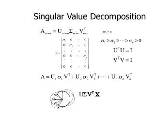
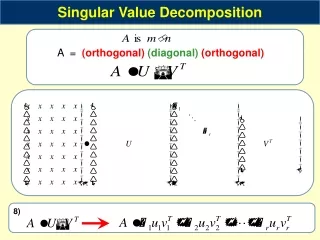
singular value decomposition UTU=I and VTV=I
suppose only pλ’s are non-zero only first p columns of U only first p columns of V
UpTUp=I and VpTVp=Isince vectors mutually pependicular and of unit length • UpUpT≠I and VpVpT≠Isince vectors do not span entire space
The part of m that lies in V0 cannot effect d since VpTV0=0 so V0 is the modelnull space
The part of d that lies in U0 cannot be affected by m • sinceΛpVpTmis multiplied byUp • and U0UpT=0 so U0 is the data null space