Download

1 / 40
400 likes | 593 Views
Winter-Weather Forecasting Topics at the WDTB Winter-Weather Workshop. Dr. David Schultz NOAA/National Severe Storms Laboratory Norman, Oklahoma schultz@nssl.noaa.gov http://www.nssl.noaa.gov/~schultz. Today’s Topics. • Rebuttal of Wetzel and Martin’s (2001) PVQ diagnostic

E N D
Winter-Weather Forecasting Topics at theWDTB Winter-Weather Workshop Dr. David Schultz NOAA/National Severe Storms Laboratory Norman, Oklahoma schultz@nssl.noaa.gov http://www.nssl.noaa.gov/~schultz
Today’s Topics • Rebuttal of Wetzel and Martin’s (2001) PVQ diagnostic • My philosophy of diagnosis • Frontogenesis - Introduction - Example 1: IPEX IOP 5 - Example 2: Elevated convection - Example 3: Midlevel NWly flow frontogenesis • Following fronts through topography (Western Region) • The melting effect (Kain et al. 2000) • One final note to cheer you up. . . .
Thoughts on Wetzel and Martin’s Ingredients-Based Methodology Specifically, PVQ. QG thinking limitations: - small grid spacings need filtered in order to interpret QG diagnostics - many nonQG processes: lake-effect, topography, convection The PVQ diagnostic: - assumes collocation of negative PV and convergence of Q (horizontally and vertically) - not clear what magnitude of PVQ means - no mathematical expression/relationship with PVQ - time constraints: if you’re going to look at the two components independently, then why look at PVQ? (cf. moisture flux convergence)
A Philosophy of Diagnosis How do we assess weather features in the atmosphere? Suppose you see something on the radar and you don’t know what is causing it. First attempt should be QG thinking: vorticity advection, warm advection, etc. If not QG, then try frontogenesis at different levels. If not frontogenesis, then something else: topography, PBL circulations, diabatic effects, etc. Note that assessing instability is also important, but secondary to this philosophy. Gravitational stability or moist symmetric instability only modulates the response to the given forcing.
Petterssen (1936) Frontogenesis F = d/dt |Ñq| F = 1/2 |Ñq| ( E cos2b - D) q = potential temperature E = resultant deformation b = angle between the isentrope and the axis of dilatation D = divergence
Frontogenesis Facts • Frontogenesis is “following the flow” (Lagrangian). • Fronts that are weakening still possess frontogenesis. • Note that tilting effects are not included in Petterssen’s (1936) form of frontogenesis. • Diagnosis of frontogenesis results in a diagnosis of the forcing for vertical motion on the frontal scale. • Ascent occurs on the warm side of a maximum of frontogenesis and on the cold side of a region of frontolysis.
Frontogenesis: Example 1 • Frontogenesis can occur even in the presence of strong topographic contrasts • In this case, from the Intermountain Precipitation Experiment, we’ll see that synoptic-scale influences can dominate over topographic influences.
IPEX IOP 5: 17 February 2000 SURFACE • Surface cyclone south of SLC • Weak flow field at all levels • Snowband northwest of cyclone • 4–12 in. snow in Tooele Valley 500 hPa
6-h median reflectivity from KMTX yellow maxima are 20-25 dBZ
700-hPa FRONTOGENESIS 500-hPa omega L 700-hPa theta shading 700-hPa frontogenesis 700-hPa winds RUC-2: 1500 UTC
Frontogenesis: Example 2 • Snowstorm in Oklahoma not well forecast • Most snowfall fell well to the north of the surface frontal boundary • Trapp et al. (2001) in March 2001 MWR
OUN SEP
Elevated Convection and Frontogenesis Frontogenesis at 1000 mb (dotted) and 600 mb (dashed) CAPE at 1000 mb (shading) and 600 mb (overprinted shading) Frontogenesis: solid lines CAPE: shading Theta-e: thin solid lines 80% RH: dotted line Heavy snow location: *
Elevated Convection and Frontogenesis circulation within plane of cross section (i.e., frontal circulation) circulation normal to plane of cross section (i.e., synoptic-scale circulation) Vertical motion: shaded Theta-es: solid lines Vertical motion: shaded Theta: solid lines
Frontogenesis: Example 3 • Frontogenesis in northwesterly flow, apparently unrelated to surface frontogenesis. • I am collecting a list of cases that look similar to this event. • Often misinterpreted as associated with upper-level jet circulations.
1300 UTC 13 Sept. 2001 surface observations, CAPE, and radar
753 J/kg CAPE 482 J/kg CIN
Tracking Cyclones and Upper-Level Forcing • Lows typically don’t move through the West continuously. • Schultz and Doswell (2000) suggested that tracking the occurrence of a mobile pressure minimum (a signal of the upper-level forcing) may assist in analysis. lee low L2 L3 Fraser River trough L1 primary low
Tracking Cyclones and Upper-Level Forcing • Look for pressure-check signatures in time series of SLP or altimeter setting, or the location of the zero isallobar
Frontal Passages in the West-I • Upstream topography tears fronts apart: Steenburgh and Mass (1996) • Fronts passing through the west can be poorly defined at the surface for many reasons. TEMPERATURE: - trapped cold air in valleys masks frontal movement aloft - diurnal heating/cooling effects - different elevations of stations (use potential temperature) - frontal retardation/acceleration by topography - precipitation (diabatic) effects - upslope/downslope adiabatic effects (e.g., Chinooks) PRESSURE: - diurnal pressure variations - sea level pressure reduction problems WINDS: - diurnal mountain/valley circulations - topography channels the wind down the pressure gradient, therefore the wind is not nearly geostrophic
Modification of Geostrophic Balance by Topography Rossby radius of deformation (lR) is a measure of the horizontal extent to which modification of the force balances takes place. lR=Nh/f lRis about 100–200 km for the Wasatch.
Blazek thesis Steenburgh and Blazek (2001)
Frontal Passages in the West-II • Warm-frontal passages are often not well defined at the surface, although regions of warm advection are likely to be occurring aloft. (Williams 1972) • “The strength of the potential temperature gradient associated with the front is strongly modulated by differential sensible heating across the front. An estimate of the contribution to frontogenesis from differential diabatic heating . . . shows that it is several times greater than the contribution from the surface winds alone.” (Hoffman 1995) • Advection of postfrontal air through the complex topography is difficult to accomplish. Therefore you may not see classic frontal passages at the surface, but the baroclinic zone may be advancing aloft. The temperature decrease (if any) behind the cold front may be a result of downward mixing of the colder air. Isallobars may be useful to follow these elevated frontal passages through the west.• Larry Dunn has described some frontal passages in the West as split fronts. This concept may be useful and is in qualitative agreement with the results described above. In these cases, the precipitation may be out ahead of the surface position of the front.
Failure of the Norwegian Cyclone Modelin Western Region • lack of warm fronts • occluded fronts sometimes act as cold fronts • deformation of fronts by topography • precipitation is often unrelated to surface features • disconnect between upper-level systems and low-level systems
The Melting Effect as a Factor in Precipitation-Type Forecasting • Kain et al. (2000): December 2000 Weather and Forecasting • Frozen precipitation falling through an above-freezing layer melts and absorbs latent heat from the environment. • If enough cooling occurs, melting precipitation can be inhibited and rain will change to snow.
1800 UTC 3 February 1998 BNA Nashville, TN
Sfc maps 44 R 42 R- 38 R- 41 R 34 S- 37 R
BNA Sounding Near-freezing isothermal layer
A shrinking bright band on radar represents a lowering melting layer, where snow changes to rain. Note how the bright band encircles the radar site (KBNA). Shrinking bright band
Important Observations • Cold advection could not explain drop in temperature. • Temperature falls were only in regions of persistent moderate precipitation. • BNA sounding showed 75-mb deep isothermal layer near 0°C. • Radar bright band was shrinking. • Surface temps did not fall below 0°C.
DT DP 500 D = – • D is the depth of precipitation needed to eliminate the melting layer (inches) • DP is the pressure depth of the above- freezing layer (mb) • DT is the mean temperature difference between the freezing point and the wet-bulb temperature of the environment (°C)
Criteria That May Warrant Consideration of the Melting Effect • Low-level temperature advection is weak. ** • Steady rainfall of at least moderate intensity is expected for several hours. • Surface temperatures are generally within a few degrees of freezing at the onset of the event.
Even if you were able to predict the liquid equivalent perfectly • . . . you’d still have to know the snow density. • Usually this is assumed to be 10 inches of snow to 1 inch of liquid water (snow ratio). • The following graph is snow ratios from 2273 snowfall events greater than 2 mm liquid from 1980–1989 for 29 U.S. stations.
10 to 1 ratio percent ratio of snow to liquid equivalent
ratios of 5–15 account for 50.8% of events percent ratio of snow to liquid equivalent