Download
1 / 15
150 likes | 297 Views
† Supported by. XXV encontro nacional de física da matéria condensada. Superconductivity in Systems with Diluted Interactions. Thereza C. de L. Paiva (IF/UFRJ), † Grzegorz Litak (TU-Lublin), Carey Huscroft (HP Co., Roseville), Raimundo R. dos Santos (IF/UFRJ), †

E N D
†Supported by XXV encontro nacional de física da matéria condensada Superconductivity in Systems with Diluted Interactions Thereza C. de L. Paiva (IF/UFRJ),† Grzegorz Litak (TU-Lublin), Carey Huscroft (HP Co., Roseville), Raimundo R. dos Santos (IF/UFRJ),† Richard T. Scalettar(UC Davis) Talk downloadable from www.if.ufrj.br/~rrds/rrds.html
Outline • Motivation • The Model • Quantum Monte Carlo • Results • Conclusions
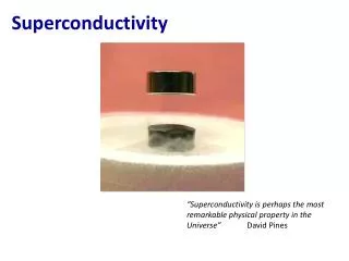
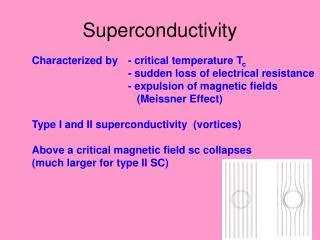
Motivation1 How much dirt (disorder) can take a super-conductor before it becomes normal (insulator or metal)? • Question even more interesting in 2-D (very thin films): • superconductivity is marginal • Kosterlitz-Thouless transition • metallic behaviour also marginal • Localization for any amount of disorder (recent expts: MIT possible?) 1 A M Goldman and N Marković, Phys. Today, Page 39, Nov 1998
t ℓ ℓ Disorder on atomic scales: sputtered amorphous films2 Sheet resistance: R at a fixed temperature can be used as a measure of disorder Mo77Ge23 film CRITICAL TEMPERATURE Tc (kelvin) independent of the size of square SHEET RESISTANCE AT T = 300K (ohms) Tc decreases with increasing disorder: screening of Coulomb repulsion is weakened 2 J Graybeal and M Beasley, PRB 29, 4167 (1984)
Metal evaporated on cold substrates, precoated with a-Ge: disorder on atomic scales.3 Bismuth System undergoes a Super-conducting - Insulator transition at T = 0 when R reaches one quantum of resistance for electron pairs, h/4e2 = 6.45 k Quantum Critical Point (evaporation without a-Ge underlayer: granular disorder on mesoscopic scales.1) 3 D B Haviland et al., PRL 62, 2180 (1989)
T Our purpose here: to understand the interplay between occupation, strength of interactions, and disorder on the SIT, through a fermion model. METAL T Tc SUC INS disorder (mag field, pressure, etc.) QCP Typical phase diagram for Quantum Critical Phenomena (any d):
The Model Use attractive Hubbard model to describe superconductivity real-space pairing Band (hopping) energy: favours fermion motion U < 0 favours on-site pairing of electrons with opposite spins Chemical pot’l: controls fermion density n Schematic phase diagram for the clean model (2D).4 Note Tc = 0 at half filling, due to coexistence of SUC with CDW. 4 RT Scalettar et al., PRL 62, 1407 (1989)
U < 0 with concentration c U = 0 with concentration f1c defects Disordered attractive Hubbard model Simple random walk arguments + time-energy uncertainty relations yield an estimate for the critical concentration of defects, f0, above which the system is an insulator:5 Dynamical, instead of purely percolative. What about dependence with filling factor? 5 G Litak and BL Gyorffy, PRB 62, 6629 (2000)
Quantum Monte Carlo6 = M auxiliary variables For the attractive model, det O = det O so there is no “minus-sign problem” Ns M x 6 W von der Linden, Phys. Rep. 220, 53 (1992); RR dos Santos, BJP (2002)
Calculated quantities, for a given realization of disorder, on an Lx L lattice: These quantities are then averaged over~ 20 - 40disorder configurations • We also need to extrapolate: • T 0 • L
c = 0.875 c = 0.625 c = 0.375 n n n Results Site occupations and Pair-field structure factor 8 8,U = 4t, T = t/(8 kB) ~ 100 K occ’n of free sites disorder Occupation of attractive sites increases with disorder Pair-field structure factor decreases with disorder (note how cdw dip at half filling disappears with increasing disorder)
Size dependence of Pair-field Structure Factor: extrapolation to the thermodynamic limit Expectation from spin-wave theory: Collecting extrapolated data for several concentrations of disorder, SUC Sp/N allows one to extract a critical fc for given temperature, n, and U.
A technical remark: • fixed such that the desired n emerges after a sequence of disorder runs (faster but leads to fluctuations in n), or • for each disorder realization choose such that the desired n emerges (slower but leads to much smaller fluctuations in n) ? Conclusion: Results are equivalent so far
Disorder-temperature section of the phase diagram Repeating the above procedures for different temperatures yields a phase diagram fc (T ), which can be inverted to yield Tc (f ) [for fixed U and n ] The theory reproduces the sharp decrease of Tc with disorder, as observed experimentally
Conclusions • Description of disordered SUC’s through random-U attractive Hubbard model seems promising • For more accurate quantitative predictions: • need to consider other fillings and interaction strengths; • need to use other quantities (e.g., current-current correlation functions) • QCP: need to go to much lower temperatures • Superconducting gap: need to examine density of states