Download
1 / 12
120 likes | 422 Views
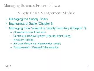
Managing Business Process Flows: Supply Chain Management Module. Managing the Supply Chain Economies of Scale (Chapter 6) Managing Flow Variability: Safety Inventory (Chapter 7) Characteristics of Forecasts Continuous Review System (Reorder Point Policy) Inventory Pooling

E N D
Managing Business Process Flows: Supply Chain Management Module • Managing the Supply Chain • Economies of Scale (Chapter 6) • Managing Flow Variability: Safety Inventory (Chapter 7) • Characteristics of Forecasts • Continuous Review System (Reorder Point Policy) • Inventory Pooling • Accurate Response (Newsvendor model) • Postponement / Delayed Differentiation
Demand uncertainty and forecasting • Forecasts depend on • historical data • “market intelligence” • Forecasts are usually (always?) wrong. • A good forecast has at least 2 numbers (includes a measure of forecast error, e.g., standard deviation). • Aggregate forecasts tend to be more accurate. • The longer the forecast horizon, the less accurate the forecast.
7.2 Safety Inventory and Service Level Example 7.1 Throughput rate Order Quantity Lead time Reorder point Definitions: Cycle service level (SL) Fill rate
Reorder Point and Cycle Service Level desired cycle service level 1.0-(desired cycle service level) SL = Prob (LTD <= ROP) MeanDemand over Leadtime Reorder Point (ROP) Reorder Point = Mean Demand over Leadtime + Safety Stock = LTD + Isafety I safety = Z * sLTD Examples 7.3 & 7.4
F(z) z 0 The standard normal distribution F(z) • Transform X = N(m,s) to z = N(0,1) • z = (X - m) / s. • F(z) = Prob( N(0,1) <z) • Transform back, knowing z*: • X* = m + z*s.
7.4 Lead Time Variability Fixed replenishment lead time • L = Supply lead time, • R=N(R, sR) =Demand per unit time is normally distributed with mean R and standard deviation sR , • Cycle service level = P(no stock out) = P(demand during lead time <ROP) = F(z*) [use tables to find z*] Safety stock Reorder point ROP = L x R + Isafety Example 7.8 (see data from 7.1)
Total variability in lead time demand = (Variability in replenishment lead time) Flow rate constant Lead time random Flow rate random Lead time fixed Example 7.9
Learning Objectives: safety stocks Safety stock increases (decreases) with an increase (decrease) in: • demand variability or forecast error, • delivery lead time for the same level of service, • delivery lead time variability for the same level of service.
7.5 The Effect of Centralization Example 7.10
Concept of Centralization • Physical Centralization • Information Centralization • Specialization • Commonality • Postponement
Learning Objectives:Centralization/pooling • Centralization reduces safety stocks (pooling) and cycle stocks (economies of scale) • Can offer better service for the same inventory investment or same service with smaller inventory investment. • Different methods to achieve pooling efficiencies: • Physical centralization,Information centralization, Specialization, Commonality, Postponement/late customization. • Cost savings are proportional to square root of # of locations pooled.
7.3 Newsvendor Problem • Marginal benefit of stocking an additional unit = MB (e.g., retail price - purchase price) • Marginal cost of stocking an additional unit = MC (e.g., purchase price - salvage price) Given an order quantity Q, increase it by one unit if and only if the expected benefit of being able to sell it exceeds the expected cost of having that unit left over. • At optimal Q, Q* = R + ZsR Data from example 7.5