IV. Sensitivity Analysis for Initial Model
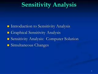
IV. Sensitivity Analysis for Initial Model. 1. Sensitivities and how are they calculated 2. Fit-independent sensitivity-analysis statistics 3. Scaled sensitivities DSS, CSS 4. Parameter correlation coefficients 5. Scaled sensitivities 1SS 6. Leverage. Sensitivities.

IV. Sensitivity Analysis for Initial Model
E N D
Presentation Transcript
IV. Sensitivity Analysis forInitial Model 1. Sensitivities and how are they calculated 2. Fit-independent sensitivity-analysis statistics 3. Scaled sensitivities DSS, CSS 4. Parameter correlation coefficients 5. Scaled sensitivities 1SS 6. Leverage
Sensitivities • Sensitivities are derivatives of dependent variables with respect to model parameters. The sensitivity of a simulated value yi’ to parameter bj is expressed as: • Sensitivities are needed by nonlinear regression to estimate parameters. • When appropriately scaled, they are also very useful by themselves. Scaling is needed because different yi’ and bj can have different units, so different values of yi’/ bj can’t always be meaningfully compared. • Can assess scaled sensitivities before performing regression, and use them to help guide the regression. “Fit-independent statistics”
Calculating sensitivities: • Sensitivity-equation sensitivities Matrix equation for heads solved by MODFLOW: Ah=f A is an nxn matrix that contains hydraulic conductivities. n=number of nodes in the grid h is an nx1 vector of heads for each node in the grid f is an nx1 vector of known quantities. Includes pumping, recharge, part of head-dependent boundary calculation, etc Take derivative with respect to parameter bj: Calculate observation sensitivities from these grid sensitivities
Calculating sensitivities: • Perturbation sensitivities forward differences or central differences y’i(bj+Δbj)- y’i(bj) y’ i(bj+Δbj)- y’ i(bj –Δbj) Δbj 2 Δbj • Sensitivities calculated using perturbation method usuallyare less accurate. • Refs: Yager, R.M. 2004; Hill & Østerby, 2003. Effects of model sensitivity and nonlinearity on parameter correlation and parameter estimation. GW flow. • UCODE and PEST: It is worth spending some time making sure the sensitivities are accurate. Work with (1) perturbation used and (2) accuracy and stability of the model. • For (2), consider solver convergence criteria and the effect of anything automatically calculated to improve solution accuracy, like time-step size for transport models. Possibly impose suitable values so they are the same for all runs used to calculate sensitivities.
Perturbation Sensitivities: forward difference Evaluation at current parameter value y’i Evaluation at increased parameter value bj
Perturbation Sensitivities: central difference Evaluation at current parameter value y’i Evaluation at increased parameter value Evaluation at decreased parameter value bj
Fit-Independent Statistics • Fit-independent statistics do not use the residual (observed minus simulated value) in the calculation of the statistic • Use sensitivities, weights, and parameter values to calculate the statistics. • Not usually presented in statistics books. They usually focus on statistics calculated after regression is complete. But when a model has a long execution time it is advantageous to do some evaluation before any regressions when the model fit may be quite poor. This is where fit-independent statistics come in.
Dimensionless Scaled Sensitivities • Dimensionless scaled sensitivity (Book, p. 48): • Indicates the amount the simulated value would change given a one-percent change in the parameter value, expressed as a percent of the observation error standard deviation (p. 49) • Can be used to compare importance of: • different observations to estimation of a single parameter. • different parameters to simulation of a single dependent variable. • Larger |dss| indicates greater importance of the observation relative to its error.
Composite Scaled Sensitivities • Composite scaled sensitivity (Book, p. 50): • CSS indicate importance of observations as a whole to a single parameter, compared with the accuracy on the observation • Can use CSS to help choose which parameters to estimate by regression. • Generally, if CSSj is more than about 2 orders of magnitude smaller than the largest CSS, it will be difficult to estimate parameter bj, and the regression may have trouble converging.
1. Composite Scaled Sensitivities Dimensionless scaled sensitivity yi = simulated observation value bj = estimated parameter value = weight of observation s = std dev of measurement error • CSS indicate importance of observations as a whole to a single parameter, compared with the accuracy on the observation • Can use CSS to help choose which parameters to estimate by regression. • Generally, if CSSj is more than about 2 orders of magnitude smaller than the largest CSS, it will be difficult to estimate parameter bj, and the regression may have trouble converging. • CSS values less than 1.0 indicate that the sensitivity contribution is less than the effect of observation error.
Exercise 4.1b • DO EXERCISE 4.1b: Use dimensionless, composite, and one-percent scaled sensitivities to evaluate observations and defined parameters. • Dimensionless scaled sensitivities for the initial steady-state model are given in Table 4-1 of Hill and Tiedeman (p. 61). • Composite scaled sensitivities are given in Table 4-1 and Figure4-3. Can be plotted with GW_Chart.
Parameter Observation Number ID HK_1 K_RB VK_CB HK_2 RCH_1 RCH_2 1 1.ss 0.11E-04 -0.225 0.105E-06 0.383E-05 0.150 0.749E-01 2 2. ss -33.3 -0.225 -0.284 -5.47 24.0 15.3 3 3. ss -57.9 -0.225 -0.493 -15.7 38.3 35.9 4 4. ss -33.3 -0.225 -0.284 -5.47 24.0 15.3 5 5. ss -46.5 -0.225 -0.394 -9.95 32.9 24.1 6 6. ss -33.4 -0.225 -0.635 -5.35 24.0 15.6 7 7. ss -2.34 -0.225 -2.38 2.08 1.82 1.04 8 8. ss -57.5 -0.225 -0.133 -16.0 37.8 36.1 9 9. ss -66.6 -0.225 -0.580E-01 -23.3 38.1 52.1 10 10. ss -46.3 -0.225 -0.330 -10.1 32.6 24.4 11 flow.ss -0.547E-03 -0.663E-04 -0.260E-05 -0.190E-03 -7.36 -3.68 Composite Scaled Sensitivity 41.3 0.214 0.783 11.0 27.4 25.6 DSS and CSS for Initial Steady-State Model Table 4-1 of Hill and Tiedeman (p. 61) Display graphically and investigate values in following slides
Why are the dss small for … • flow01.ss • hd07.ss • hd01.ss hd01.ss flow01.ss hd01.ss
CSS for Initial Steady-State Model Figure 4-3 of Hill and Tiedeman (p. 62)
Parameter Correlation Coefficients • Parameter correlation coefficients are a measure of whether or not the calibration data can be used to estimateindependently each of a pair of parameters. • It is important that the sensitivity analysis of the initial model include an assessment of the parameter correlation coefficients. • We will intuitively assess the correlation coefficients here, and more rigorously explain them later in the course. • DO EXERCISE 4.1c: Use parameter correlation coefficients to assess parameter uniqueness. • The parameter correlation coefficient matrix for the starting parameter values for the steady-state problem, calculated using the hydraulic-head and flow observations, is shown in Table 4-2 of Hill and Tiedeman (p. 62). The parameter correlation coefficient matrix calculated using only the hydraulic-head data is shown in Table 4-3 (p. 63).
HK_1 K_RB VK_CB HK_2 RCH_1 RCH_2 HK_1 1.00 -0.37 -0.57 -0.75 0.95 -0.63 K_RB 1.00 -0.11 0.31 -0.22 0.25 VK_CB 1.00 0.82 -0.68 0.81 HK_2 symmetric 1.00 -0.83 0.98 RCH_1 1.00 -0.76 RCH_2 1.00 Parameter Correlation Coefficients • Calculated by MODFLOW-2000, using head and flow data. Table 4-2A of Hill and Tiedeman (p. 62)
HK_1 K_RB VK_CB HK_2 RCH_1 RCH_2 HK_1 1.00 1.00 1.00 1.00 1.00 1.00 K_RB 1.00 1.00 1.00 1.00 1.00 VK_CB 1.00 1.00 1.00 1.00 HK_2 symmetric 1.00 1.00 1.00 RCH_1 1.00 1.00 RCH_2 1.00 Parameter Correlation Coefficients • Calculated by MODFLOW-2000, using only head data. Table 4-3A of Hill and Tiedeman (p. 73)
HK_1 K_RB VK_CB HK_2 RCH_1 RCH_2 HK_1 1.00 0.97 1.00 1.00 1.00 1.00 K_RB 1.00 0.97 0.97 0.97 0.97 VK_CB 1.00 1.00 1.00 1.00 HK_2 symmetric 1.00 1.00 1.00 RCH_1 1.00 1.00 RCH_2 1.00 Parameter Correlation Coefficients • Calculated by UCODE_2005, using only head data. Table 4-3B of Hill and Tiedeman (p. 63)
One-Percent Scaled Sensitivities • One-percent scaled sensitivity (Book, p. 54): • In units of the observations; can be thought of as change in simulated value due to 1% increase in parameter value. • One-percent is used because for nonlinear models, sensitivities change with parameter value. Sensitivities are likely to be less accurate far from the parameter values at which they are calculated. • These dimensional quantities can sometimes be used to convey the sensitivity information in a more meaningful way than the dimensionless scaled sensitivities. • Can be used to create contour maps of one-percent scaled sensitivities for hydraulic heads in a given model layer.
One-Percent Sensitivity Maps For Initial Model • One-percent sensitivity maps of hydraulic head to a model parameter can provide useful information about a simulated flow system. • For the simple steady-state model used in these exercises, the one-percent sensitivity maps can be explained using Darcy’s Law and the simulated fluxes of the simple flow system. • DO EXERCISE 4.1d: Evaluate contour maps of one-percent sensitivities for the steady-state flow system. • These maps are shown in Figure 4-4 of Hill and Tiedeman (p. 64).
One-Percent Sensitivities for HK_1 Figure 4-4A of Hill and Tiedeman Zero at river. Why? Negative away from river. Why? Contours closer near the river. Why? Values in layers 1 and 2 similar. Why?
One-Percent Sensitivities for K_RB Figure 4-4C of Hill and Tiedeman Constant over the whole system. Why?
One-Percent Sensitivities for RCH_1 Figure 4-4E of Hill and Tiedeman Constant on right side of system. Why?
One-Percent Sensitivities for RCH_2 Figure 4-4F of Hill and Tiedeman Contours equally spaced on left side of system. Why?
Leverage • Leverage statistics reflect the effects of DSS and parameter correlation coefficients. • Exercise 4.1e
hd01, hd07, flow01 important because their effects of parameter correlation. Hd09.ss important because of high sensitivities.