Download
1 / 8
80 likes | 189 Views
This study explores the ocean's significant contribution (about one-third) to atmospheric mercury emissions, highlighting uncertainties in the flux's magnitude, seasonality, and distribution. It analyzes factors influencing ocean-atmosphere cycling of mercury, including radiation, primary productivity, and mixed layer depth. By comparing modeled ocean flux data with observations, the research identifies seasonal patterns and spatial variability in mercury concentrations. The findings emphasize the need for further studies to refine our understanding of ocean emissions and their impact on global mercury transport and concentration trends.

E N D
Role of Ocean Emissions in the Mercury Budget Sarah Strode, Lyatt Jaeglé Department of Atmospheric Sciences, University of Washington Noelle Eckley Selin, Rokjin Park, Daniel Jacob Department of Earth and Planetary Sciences, Harvard University
The ocean in the global Hg budget • The ocean represents about a third of the total source to the atmosphere • The magnitude, seasonality, and distribution of the flux are still uncertain • reemits deposited mercury role in global transport From Mason and Sheu, 2002
Ocean-atmosphere cycling of Hg0 • Reduction proportional to radiation and net primary productivity (MODIS 2003) • d[HgII]aq/dt = deposition – Kl*[HgII]aq – Kr*[HgII]aq • d[Hg0]aq/dt = Kr*[HgII]aq – Kw([Hg0]aq – H*[Hg0]atmos) • Evasion based on kw=f(T,u102) and H=f(T) • Loss and reduction scaled together to yield total flux=2000 Mg/yr transport Hg0 HgII oxidation MLD from NRL mixed layer depth climatology Marine Boundary Layer Evasion (T,wind) deposition t =7 months (4-79 months) reduction Hg0 HgII P(light,biology) Surface ocean Loss t =7 months
Observed & modeled total aqueous Hg June-Aug Sept-Oct Dec-Feb March-May pM Observations from: Coquery & Cossa 1995, Cossa et al. 2004, Dalziel 1995, Ferrara et al. 2003, Gill & Fitgerald 1987, Kim & Fitgerald 1986, Laurier et al. 2004, Mason & Fitgerald 1993, Mason et al. 1998, Mason et al. 2001, Mason & Sullivan 1999
Comparison to Observations DGM (pM) Ocean Flux (ng/m2/h) 1.5 1.0 0.5 0 12 8 4 0 Med. Sea N. Atl. eq. Pac Baltic eq. Pac N. Atl. JJA JJA JJA MAM DJF SON Med. Sea N. Atl. N. Atl. Baltic Pacific JJA SON JJA MAM MAM Observation Observations from: Baeyens & Leermakers 1998, Coquery & Cossa 1995, Gardfeldt et al. 2003, Kim & Fitzgerald 1986, Laurier et al. 2003, Mason & Fitzgerald 1994, Mason et al. 1998, Wangberg et al. 2001 Model
Ocean flux distribution & seasonality Jan. ocean flux July ocean flux 0 100 200 300 kg July • Higher flux in tropics due to high temperature and radiation • High flux in regions of high deposition • Seasonality due to temperature, npp, radiation, and mixed layer depth Jan. latitude
Effect of Ocean Flux Annual Hg0 surface concentration Monthly ocean source contribution • Ocean source: 40-50% of surface Hg0 over the southern ocean • 15-35% over northern continents • Seasonal variability due to seasonality of ocean source % S. Pacific N. America Europe ng/m3 Contribution of Ocean Source % %
Summary • Model captures some of the spatial and temporal variability in ocean mercury concentrations and fluxes, but misses the extreme values seen in observations • The ocean flux shows a large seasonal cycle and spatial variability due to the variability in mixed layer depth, radiation, npp, temperature, and deposition • Future work: continue comparing model seasonality to observations of atmospheric concentrations at coastal sites