3 rd Homework Solution
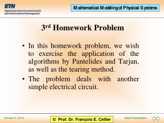
In this homework problem, we wish to exercise the application of the algorithms by Pantelides and Tarjan, as well as the tearing method. The problem deals with another simple electrical circuit. 3 rd Homework Solution. Structural Singularity Pantelides Algorithm Tarjan Algorithm

3 rd Homework Solution
E N D
Presentation Transcript
In this homework problem, we wish to exercise the application of the algorithms by Pantelides and Tarjan, as well as the tearing method. The problem deals with another simple electrical circuit. 3rd Homework Solution
Structural Singularity Pantelides Algorithm Tarjan Algorithm Tearing of Algebraic Loops Structure Diagram Solving of Coupled Equations
iC2 iR1 iR2 iR4 v1 v3 v4 v2 iR3 iC3 iC1 i0 v0 Structural Singularity Show that the circuit depicted on the left exhibits a structural singularity. To this end, find a complete set of equations in currents, potentials, and Voltages (ignoring the mesh equations), and draw the digraph of the resulting DAE system. Subsequently, color the digraph by use of the algorithm by Tarjan, and demonstrate that the system is indeed structurally singular. Explain the structural singularity by analyzing the mesh that is formed by the three capacitors.
1: U0 = f(t)13: U0 = v1 – v0 2: uR1 = R1 · iR1 14: uR1 = v1 – v2 3: uR2 = R2 · iR2 15: uR2 = v2 – v3 4: uR3 = R3 · iR3 16: uR3 = v3 – v0 5: uR4 = R4 · iR4 17: uR4 = v3 – v4 6: iC1 = C1 · duC1 /dt 18:uC1 = v2 – v0 7: iC2 = C2 · duC2 /dt 19:uC2 = v2 – v4 8: iC3 = C3 · duC3 /dt 20:uC3 = v4 – v0 9:i0 = iR1 21:v0 = 0 10:iR1 = iC1 + iC2 + iR2 11:iR2 = iR3 + iR4 12:iC3 = iR4 + iC2 U0 i0 uR1 iR1 uR2 iR2 uR3 iR3 uR4 iR4 duC1/dt iC1 duC2/dt iC2 duC3/dt iC3 v0 v1 v2 v3 v4 01 02 03 04 05 06 07 08 09 10 11 12 13 14 15 16 17 18 19 20 21
1:U0 = f(t)13:U0 = v1 – v0 2: uR1 = R1 · iR1 14: uR1 = v1 – v2 3: uR2 = R2 · iR2 15: uR2 = v2 – v3 4: uR3 = R3 · iR3 16: uR3 = v3 – v0 5: uR4 = R4 · iR4 17: uR4 = v3 – v4 6:iC1 = C1 · duC1 /dt18:uC1 = v2 – v0 7:iC2 = C2 · duC2 /dt19:uC2 = v2 – v4 8:iC3 = C3 · duC3 /dt20:uC3 = v4 – v0 9:i0 = iR121:v0 = 0 10:iR1 = iC1 + iC2 + iR2 11:iR2 = iR3 + iR4 12:iC3 = iR4 + iC2 U0 i0 uR1 iR1 uR2 iR2 uR3 iR3 uR4 iR4 duC1/dt iC1 duC2/dt iC2 duC3/dt iC3 v0 v1 v2 v3 v4 01 02 03 04 05 06 07 08 09 10 11 12 13 14 15 16 17 18 19 20 21
1:U0 = f(t)13:U0 = v1 – v0 2: uR1 = R1 · iR1 14: uR1 = v1 – v2 3: uR2 = R2 · iR2 15: uR2 = v2 – v3 4: uR3 = R3 · iR3 16: uR3 = v3 – v0 5: uR4 = R4 · iR4 17: uR4 = v3 – v4 6:iC1 = C1 · duC1 /dt18:uC1 = v2 – v0 7:iC2 = C2 · duC2 /dt19:uC2 = v2 – v4 8:iC3 = C3 · duC3 /dt20:uC3 = v4 – v0 9:i0 = iR121:v0 = 0 10:iR1 = iC1 + iC2 + iR2 11:iR2 = iR3 + iR4 12:iC3 = iR4 + iC2 U0 i0 uR1 iR1 uR2 iR2 uR3 iR3 uR4 iR4 duC1/dt iC1 duC2/dt iC2 duC3/dt iC3 v0 v1 v2 v3 v4 01 02 03 04 05 06 07 08 09 10 11 12 13 14 15 16 17 18 19 20 21 Constraint equation
Apply the algorithm by Pantelides to the equation system found before, and determine the resulting DAE system that by now no longer exhibits any structural singularity. Find the structure incidence matrix of the resulting implicit DAE system. Pantelides Algorithm
U0 i0 uR1 iR1 uR2 iR2 uR3 iR3 uR4 iR4 duC1/dt iC1 duC2 iC2 duC3/dt iC3 v0 v1 v2 v3 v4 uC2 dv0 dv2 dv4 01 02 03 04 05 06 07 08 09 10 11 12 13 14 15 16 17 18 19 20 21 22 23 24 25 1:U0 = f(t)13:U0 = v1 – v0 2: uR1 = R1 · iR1 14: uR1 = v1 – v2 3: uR2 = R2 · iR2 15: uR2 = v2 – v3 4: uR3 = R3 · iR3 16: uR3 = v3 – v0 5: uR4 = R4 · iR4 17: uR4 = v3 – v4 6:iC1 = C1 · duC1 /dt18:uC1 = v2 – v0 7:iC2 = C2 · duC219:uC2 = v2 – v4 8:iC3 = C3 · duC3 /dt20:uC3 = v4 – v0 9:i0 = iR121:v0 = 0 10:iR1 = iC1 + iC2 + iR2 22:duC2 = dv2 – dv4 11:iR2 = iR3 + iR4 23:duC1 /dt = dv2 – dv0 12:iC3 = iR4 + iC2 24:duC3 /dt = dv4 – dv0 25:dv0 = 0
Draw the digraph of the resulting DAE system, and color it by use of the algorithm by Tarjan. The colored digraph symbolizes a partially sorted equation system, which however still contains a large algebraic loop. Write down the partially sorted equation system. Find the structure incidence matrix of the partially sorted equation system. This is now in block lower triangular form ( BLT-Form). Algorithm by Tarjan
U0 i0 uR1 iR1 uR2 iR2 uR3 iR3 uR4 iR4 duC1/dt iC1 duC2 iC2 duC3/dt iC3 v0 v1 v2 v3 v4 uC2 dv0 dv2 dv4 01 09 03 04 05 06 07 08 25 10 11 12 03 08 15 16 17 04 06 05 02 22 23 24 07 01:U0 = f(t)03:U0 = v1 – v0 09:uR1 = R1 · iR108:uR1 = v1 – v2 3: uR2 = R2 · iR2 15: uR2 = v2 – v3 4: uR3 = R3 · iR3 16: uR3 = v3 – v0 5: uR4 = R4 · iR4 17: uR4 = v3 – v4 6:iC1 = C1 · duC1 /dt04:uC1 = v2 – v0 7:iC2 = C2 · duC206:uC2 = v2 – v4 8:iC3 = C3 · duC3 /dt05:uC3 = v4 – v0 25:i0 = iR102:v0 = 0 10:iR1 = iC1 + iC2 + iR2 22:duC2 = dv2 – dv4 11:iR2 = iR3 + iR4 23:duC1 /dt = dv2 – dv0 12:iC3 = iR4 + iC2 24:duC3 /dt = dv4 – dv0 07:dv0 = 0
Find appropriate tearing variables using the following heuristics: Tearing of the Algebraic Loop In the digraph, determine those equations with the largest number of unknowns. For every one of these equations, find those unknowns that show up most frequently in the not yet used equations. For every one of these variables, determine how many additional equations can be made causal if they are assumed known. Choose the one variable as the next tearing variable, which allows to make the largest number of additional equations causal.
1st tearing variable Selection of tearing variables: Equations: 10 11 12 22 (all with 3 variables each) iR2 iC1 iC2 duC2 dv2 dv4 2 eq. 2 eq. 2 eq. 3 eq. 2 eq. 3 eq. iR2 iR3 iR4 iR4 iC2 iC3 3 eq. 2 eq. 3 eq. 3 eq. 3 eq. 2 eq.
U0 i0 uR1 iR1 uR2 iR2 uR3 iR3 uR4 iR4 duC1/dt iC1 duC2 iC2 duC3/dt iC3 v0 v1 v2 v3 v4 uC2 dv0 dv2 dv4 01 09 03 04 05 06 07 08 25 10 10 12 03 08 15 16 17 04 06 05 02 22 23 24 07 01:U0 = f(t)03:U0 = v1 – v0 09:uR1 = R1 · iR108:uR1 = v1 – v2 3: uR2 = R2 · iR215: uR2 = v2 – v3 4: uR3 = R3 · iR3 16: uR3 = v3 – v0 5: uR4 = R4 · iR4 17: uR4 = v3 – v4 6:iC1 = C1 · duC1 /dt04:uC1 = v2 – v0 7:iC2 = C2 · duC206:uC2 = v2 – v4 8:iC3 = C3 · duC3 /dt05:uC3 = v4 – v0 25:i0 = iR102:v0 = 0 10:iR1 = iC1 + iC2 + iR222:duC2 = dv2 – dv4 10: iR2 = iR3 + iR4 23:duC1 /dt = dv2 – dv0 12:iC3 = iR4 + iC2 24:duC3 /dt = dv4 – dv0 07:dv0 = 0
U0 i0 uR1 iR1 uR2 iR2 uR3 iR3 uR4 iR4 duC1/dt iC1 duC2 iC2 duC3/dt iC3 v0 v1 v2 v3 v4 uC2 dv0 dv2 dv4 01 09 11 15 16 06 07 08 25 10 10 12 03 08 12 13 14 04 06 05 02 22 23 24 07 01:U0 = f(t)03:U0 = v1 – v0 09:uR1 = R1 · iR108:uR1 = v1 – v2 11: uR2 = R2 · iR212:uR2 = v2 – v3 15:uR3 = R3 · iR313: uR3 = v3 – v0 16:uR4 = R4 · iR414: uR4 = v3 – v4 6:iC1 = C1 · duC1 /dt04:uC1 = v2 – v0 7:iC2 = C2 · duC206:uC2 = v2 – v4 8:iC3 = C3 · duC3 /dt05:uC3 = v4 – v0 25:i0 = iR102:v0 = 0 10:iR1 = iC1 + iC2 + iR222:duC2 = dv2 – dv4 10: iR2 = iR3 + iR423:duC1 /dt = dv2 – dv0 12:iC3 = iR4 + iC2 24:duC3 /dt = dv4 – dv0 07:dv0 = 0
2nd tearing variable Selection of tearing variables: Equations: 22 (the only equation with 3 unknowns) duC2 dv2 dv4 2 eq. 2 eq. 2 eq.
U0 i0 uR1 iR1 uR2 iR2 uR3 iR3 uR4 iR4 duC1/dt iC1 duC2 iC2 duC3/dt iC3 v0 v1 v2 v3 v4 uC2 dv0 dv2 dv4 01 09 11 15 16 06 07 08 25 10 10 12 03 08 12 13 14 04 06 05 02 17 23 24 07 01:U0 = f(t)03:U0 = v1 – v0 09:uR1 = R1 · iR108:uR1 = v1 – v2 11: uR2 = R2 · iR212:uR2 = v2 – v3 15:uR3 = R3 · iR313: uR3 = v3 – v0 16:uR4 = R4 · iR4 14: uR4 = v3 – v4 6:iC1 = C1 · duC1 /dt04:uC1 = v2 – v0 7:iC2 = C2 · duC206:uC2 = v2 – v4 8:iC3 = C3 · duC3 /dt05:uC3 = v4 – v0 25:i0 = iR102:v0 = 0 10:iR1 = iC1 + iC2 + iR217:duC2 = dv2 – dv4 10: iR2 = iR3 + iR423:duC1 /dt = dv2 – dv0 12:iC3 = iR4 + iC2 24:duC3 /dt = dv4 – dv0 07:dv0 = 0
U0 i0 uR1 iR1 uR2 iR2 uR3 iR3 uR4 iR4 duC1/dt iC1 duC2 iC2 duC3/dt iC3 v0 v1 v2 v3 v4 uC2 dv0 dv2 dv4 01 09 11 15 16 21 18 22 25 19 10 20 03 08 12 13 14 04 06 05 02 17 23 24 07 01:U0 = f(t)03:U0 = v1 – v0 09:uR1 = R1 · iR108:uR1 = v1 – v2 11: uR2 = R2 · iR212:uR2 = v2 – v3 15:uR3 = R3 · iR313: uR3 = v3 – v0 16:uR4 = R4 · iR414: uR4 = v3 – v4 21:iC1 = C1 · duC1 /dt04:uC1 = v2 – v0 18:iC2 = C2 · duC206:uC2 = v2 – v4 22:iC3 = C3 · duC3 /dt05:uC3 = v4 – v0 25:i0 = iR102:v0 = 0 19:iR1 = iC1 + iC2 + iR217:duC2 = dv2 – dv4 10: iR2 = iR3 + iR423:duC1 /dt = dv2 – dv0 20:iC3 = iR4 + iC224:duC3 /dt = dv4 – dv0 07:dv0 = 0
U0 i0 uR1 iR1 uR2 iR2 uR3 iR3 uR4 iR4 duC1/dt iC1 duC2 iC2 duC3/dt iC3 v0 v1 v2 v3 v4 uC2 dv0 dv2 dv4 01 09 11 15 16 21 18 22 25 19 10 20 03 08 12 13 14 04 06 05 02 17 23 24 07 01:U0 = f(t)14: uR4 = v3 – v4 02:v0 = 0 15: iR3 = uR3 /R3 03:v1 = U0 – v016: iR4 = uR4 /R4 04:v2 = uC1 – v017:duC2 = dv2 – dv4 05:v4 = uC3 – v018:iC2 = C2 · duC2 06:uC2 = v2 – v419:iC1= iR1–iC2–iR2 07:dv0 = 0 20:iC3 = iR4 + iC2 08:uR1 = v1 – v221:duC1 /dt = iC1 /C1 09:iR1 = uR1 /R122:duC3 /dt = iC3 /C3 10: iR2 = iR3 + iR423:dv2= duC1 /dt – dv0 11: uR2 = R2 · iR2 24:dv4= duC3 /dt – dv0 12: v3 = v2 – uR225:i0 = iR1 13: uR3 = v3 – v0
Draw the structure diagram of the causalized algebraic loop. It can be seen that two tearing variables are needed to make all equations of the loop causal. The two tearing variables decouple the equation system in such a way that there result two separate equation systems in one tearing variable each (this is not always the case, but it happens in the given example). Find the structure incidence matrix of the fully causalized DAE system. This now has two diagonal blocks of smaller sizes. Structure Diagram
v3 Algebraic Loop dv4 iC2 iC3 dv2 iC1 uR4 iR4 uR3 uR2 iR3 1st tearing variable duC2 duC3 /dt duC1 /dt 2nd tearing variable iR2
Solve the two equation systems symbolically, and replace the residual equations of the equation system by the so found explicit equations. Draw the digraph of the once more modified equation system, and color it by use of the algorithm by Tarjan. Determine the resulting structure incidence matrix. This is now in lower triangular form. Solving the Coupled Equations
iR2 = iR3 + iR4 01:U0 = f(t)14: uR4= v3 – v4 02:v0 = 0 15: iR3= uR3 /R3 03:v1 = U0 – v016: iR4= uR4 /R4 04:v2 = uC1 – v017:duC2 = dv2 – dv4 05:v4 = uC3 – v018:iC2 = C2 · duC2 06:uC2 = v2 – v419:iC1= iR1–iC2–iR2 07:dv0 = 0 20:iC3 = iR4 + iC2 08:uR1 = v1 – v221:duC1 /dt = iC1 /C1 09:iR1 = uR1 /R122:duC3 /dt = iC3 /C3 10: iR2= iR3 + iR423:dv2= duC1 /dt – dv0 11: uR2= R2 · iR2 24:dv4= duC3 /dt – dv0 12: v3= v2 – uR225:i0 = iR1 13: uR3= v3 – v0 = uR3 /R3 + uR4 /R4 = (v3 – v0)/R3 + (v3 – v4)/R4 = (R3 + R4 )/(R3·R4 ) v3– v0 /R3 – v4 /R4 = (R3 + R4 )/(R3·R4 ) · (v2 – uR2 )– v0 /R3 – v4 /R4 = – (R3 + R4 )/(R3·R4 ) · uR2 + (R3 + R4 )/(R3·R4 ) · v2 – v0 /R3 – v4 /R4 = – R2 · (R3 + R4 )/(R3·R4 ) · iR2 + (R3 + R4 )/(R3·R4 ) · v2 – v0 /R3 – v4 /R4 (R3 + R4 ) · v2 – R4 · v0 – R3 · v4 iR2 = R2·R3 + R2·R4 + R3·R4
duC2 = dv2 – dv4 01:U0 = f(t)14: uR4= v3 – v4 02:v0 = 0 15: iR3= uR3 /R3 03:v1 = U0 – v016: iR4= uR4 /R4 04:v2 = uC1 – v017:duC2 = dv2 – dv4 05:v4 = uC3 – v018:iC2 = C2 · duC2 06:uC2 = v2 – v419:iC1= iR1–iC2–iR2 07:dv0 = 0 20:iC3 = iR4 + iC2 08:uR1 = v1 – v221:duC1 /dt = iC1 /C1 09:iR1 = uR1 /R122:duC3 /dt = iC3 /C3 10: iR2 = iR3 + iR423:dv2= duC1 /dt – dv0 11: uR2= R2 · iR2 24:dv4= duC3 /dt – dv0 12: v3= v2 – uR225:i0 = iR1 13: uR3= v3 – v0 = (duC1 /dt – dv0) – (duC3 /dt – dv0) = duC1 /dt – duC3 /dt = iC1 /C1 – iC3 /C3 = (iR1–iC2–iR2 )/C1 – (iR4 + iC2)/C3 = – (C1 + C3 )/(C1 · C3 ) · iC2 + (iR1–iR2 )/C1 – iR4 /C3 = – C2 · (C1 + C3 )/(C1 · C3 ) · duC2 + (iR1–iR2 )/C1 – iR4 /C3 C3 · (iR1–iR2 )– C1 · iR4 duC2 = C1·C2 + C1·C3 + C2·C3
01:U0 = f(t) 02:v0 = 0 03:v1 = U0 – v0 04:v2 = uC1 – v0 05:v4 = uC3 – v0 06:uC2 = v2 – v4 07:dv0 = 0 08:uR1 = v1 – v2 09:iR1 = uR1 /R1 10: 11:uR2 = R2 · iR2 12:v3= v2 – uR2 13:uR3 = v3 – v0 14:uR4 = v3– v4 15:iR3 = uR3 /R3 16:iR4 = uR4 /R4 17: 18:iC2 = C2 · duC2 19:iC1= iR1–iC2–iR2 20:iC3 = iR4 + iC2 21:duC1 /dt = iC1 /C1 22:duC3 /dt = iC3 /C3 23:dv2= duC1 /dt – dv0 24:dv4= duC3 /dt – dv0 25:i0 = iR1 (R3 + R4 ) · v2 – R4 · v0 – R3 · v4 C3 · (iR1–iR2)– C1 · iR4 duC2 = iR2 = C1·C2 + C1·C3 + C2·C3 R2·R3 + R2·R4 + R3·R4
U0 i0 uR1 iR1 uR2 iR2 uR3 iR3 uR4 iR4 duC1/dt iC1 duC2 iC2 duC3/dt iC3 v0 v1 v2 v3 v4 uC2 dv0 dv2 dv4 U0 i0 uR1 iR1 uR2 iR2 uR3 iR3 uR4 iR4 duC1/dt iC1 duC2 iC2 duC3/dt iC3 v0 v1 v2 v3 v4 uC2 dv0 dv2 dv4 01 09 11 15 16 21 18 22 25 19 10 20 03 08 12 13 14 04 06 05 02 17 23 24 07 01 09 11 15 16 21 18 22 25 19 10 20 03 08 12 13 14 04 06 05 02 17 23 24 07