Download
1 / 49
490 likes | 537 Views
Explore the roadmap to realism in computer graphics, from geometry and rendering to interactive behavior. Learn about trade-offs, balancing costs and quality in achieving realistic visuals in various media and applications.

E N D
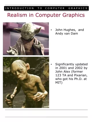
Realism in Computer Graphics • John Hughes, and Andy van Dam • Significantly updated in 2001 and 2002 by John Alex (former 123 TA and Pixarian, who got his Ph.D. at MIT)
Realism in Computer Graphics Roadmap • We tend to mean physical realism • How much can you deliver? • what medium? (still images, movie/video special effects, etc.) • what resources are you willing to spend? (time, money, processing power) • How much do you want or need? Depends on: • content (movies, scientific visualization, etc) • users (experts vs. novice) • The many categories of realism: • geometry and modeling • rendering • behavior • interaction • Many techniques for achieving varying amounts of realism within each category • Achieving realism usually requires trade-offs • realistic in some categories, not in others • concentrate on the aspects most useful to your application
Realism and Media (1/2) What is “realism”? • King Kong (1933) vs. King Kong (2005) • In the early days of computer graphics, focus was primarily directed towards producing still images • “realism” typically meant approaching “photorealism.” Goal: to accurately reconstruct a scene at a particular slice of time • Emphasis placed on accurately modeling geometry and light reflection properties of surfaces • With the increasing production of animated graphics (commercials, movies, special effects, cartoons) new standard of “realism” important: • Behavior over time: • character animation • natural phenomena: cloth, fur, hair, skin, smoke, water, clouds, wind • Newtonian physics: things that bump, collide, fall, scatter, bend, shatter, etc. • Some of which is now calculated on a dedicated physics card! (eg. AGEIA PhysX)
Realism and Media (2/2) Real-time vs. Non-real-time • “Realistic” static images and animations are rendered in batch and viewed later. They often take hours per frame to produce. Time is a relatively unlimited resource • In contrast, other apps emphasize real-time output: • graphics workstations: data visualization, 3D design • video games • virtual reality • Any media that involves user interaction (e.g., all of the above) also requires real-time interaction handling Rendered image Real-time interaction
Trade-offs (1/5) Cost vs. Quality • Many computer graphics media (e.g., film vs. video vs. CRT) • Many categories of realism to consider (far from exhaustive): • geometry • behavior • rendering • interaction • Worst-case scenario: must attend to all of these categories within an extremely limited time-budget • Optimal balance of techniques for achieving “realism” highly depends on context of use: • medium • user • content • resources (especially hardware) • We will elaborate on these four points next…
Trade-offs (2/5) • Medium • Different media --> different needs • Consider: doctor examining x-rays: • if examining static transparencies, resolution and accuracy matter most • if doctor is interactively browsing a 3D dataset of the patient’s body online, may want to sacrifice resolution or accuracy for faster navigation and ability to zoom in at higher resolution on regions of interest • User • Expert vs. novice users • Data visualization: • novice may see a clip of data visualization on the news, doesn’t care about fine detail (e.g., weather maps) • expert at workstation will examine details and stumble over artifacts and small errors—“expertise” involves acute sensitivity to small fluctuations in data, anomalies, patterns, features • in general, “what does the user care (most) about?”
Trade-offs (3/5) Content • movie special-effects pack as much astonishment as possible into budget: every trick in book • conversely, CAD model rendering typically elides detail for clarity, and fancy effects interfere with communication • Scientific visualizations show artifacts and holes in data, don’t smooth them out.
Trade-offs (4/5) Resources • Intel 286 (1989) • wireframe bounding boxes • Microsoft Xbox360 (2006) • Tri-core (3*3.2Ghz) system with onboard ATI graphics hardware – capable of 1080p HDTV output – complete with controllers for $350 • nVidia GeForce 8800GTX (2006) • texture-mapped, environment-mapped, bump-mapped, shadow-mapped, 11 billion vertices/second, subsurface scattering, stencil-shadowed goodness for $600 fully loaded • AGEIA PhysX (2005) • Explosions, dust, cloth, smoke, fog, lifelike character animation for an extra $150
Trade-offs (5/5) Computing to a time budget (“time-critical” algos) • A vast array of techniques have been developed for generating “realistic” geometry, behavior, rendering… • The “best” can often be traded for the “good” at a much lower computational price • We call bargain-basement deals “hacks” • Some techniques use progressive refinement (or its inverse, graceful degradation): the more time we spend, the better output we get. • Excellent for situations when we want the best quality output we can get for a fixed period of time, but we can’t overshoot our time limit (e.g., IVR surgery!). Maintaining constant update rates is a form of guaranteed “Quality of Service” (a networking term). • web image downloads • progressive refinement for extremely large meshes • see also slide 11 and 14… http://www.equinox3d.com/renderer.html
Digression - Definitions • Texture-Maps: map an image onto surface geometry to create appearance of fine surface detail. A high level of realism may require many layers of textures. • Environment-Maps: multiple images (textures) which record global reflection and lighting on object. These images are resampled during rendering to extract view- specific information which is then applied as texture to object. • Bump-Maps: fake surface normals by applying height field (intensities in the map indicate height above surface). From height field calculate gradient across surface and use this to perturb the surface normal. • Normal-Maps: similar to bump-maps. Instead of using grayscale image to calculate the normals, pre-generate normals from high-resolution model and store result in the low-resolution polygonal model. • Shadow-Maps: generate shadow texture by capturing silhouettes of objects as seen from the light source. Project texture onto scene. Note: must recalculate for moving lights.
Mesh decimation: Techniques—Geometry (1/4) • The Hacked • Texture mapping: excellent way to fake fine surface detail—more often used to fake geometry than to add pretty colors • more complicated texture mapping strategies such as polynomial texture maps use image-based techniques for added realism • The Good • Polygonization: very finely tessellated meshings of curved surfaces • Polys easily converted to subdivisional surfaces (right). More on this later. • linear approximation • massively hardware-accelerated!
Techniques—Geometry (2/4) The Best • Splines • no polygons at all! Continuous mathematical surface representations (polynomials) • 2D and 3D curved surfaces: Non-Uniform Rational B-Splines (NURBS) • control points • high order polynomials are hard to work with • used a lot in computer-aided designs, engineering • Implicit Surfaces (blobbies) • F(x,y,z) = 0 • add, subtract, blend • relatively hard to render (need to raytrace or convert to polygon, both slow) F(x,y,z) = ((x^2*(1-x^2)-y^2)^2+0.5*z^2-f*(1+b*(x^2+y^2+z^2)) = 0
Techniques—Geometry (3/4) The Best • Subdivision Surfaces • subdivide triangles into more triangles, moving to a continuous limit surface • elegantly avoid gapping and tearing between features • support creases • allow multi-resolution deformations (editing of lower resolution representation of surface) From Pixar’s “Geri’s Game”
Techniques—Geometry (4/4) • The Gracefully Degraded • Level-of-Detail(LOD): as object gets farther away from viewer, replace it with a lower-polygon version or lower quality texture map. Discontinuous jumps in model detail • Mesh decimation:save polygons Left: 30,392 triangles Right: 3,774 triangles
Techniques—Rendering (1/9) Good Hacks • Easily implemented in hardware: fast! • Use polygons • Only calculate lighting at polygon vertices, from point lights • For non-specular (i.e., not perfectly reflective), opaque objects, most light comes directly from the lights (“locally”), and not “globally” from other surfaces in the scene • Local lighting approximations • diffuse Lambertian reflection: only accounts for angle between surface normal and vectors to the light source. • fake specular spots on shiny surfaces: Phong lighting • Global lighting approximations • introduce a constant “ambient” lighting term to fake an overall global contribution • reflection: environment mapping • shadows: shadow mapping • Polygon interior pixels shaded by simple color interpolation: Gouraud shading • Phong shading: evaluate some lighting functions on a per-pixel basis, using interpolated surface normal.
Techniques—Rendering (2/9) Example: Doom 3 • Few polygons (i.e., low geometric complexity (a.k.a. scene complexity)) • Purely local lighting calculations • Details created by texturing everything with precomputed texture maps • surface detail • smoke, contrails, damage and debris • even the lighting and shadows are done with textures • “sprites” used for flashes and explosions • Bump mapping in hardware
Techniques—Rendering (3/9) The Best • Global illumination: find out where all the light entering a scene comes from, where and how much it is absorbed, reflected or refracted, and all the places it eventually winds up • We cover Ray-tracing (specular) and Radiosity (diffuse), neither is physically accurate. • IBR. Not geometry-based, explained later under Image-Based Rendering. • Early method: Ray-tracing. Avoid forward tracing infinitely many light rays from light sources to eye. Work backwards to do viewer/pixel-centric rendering: shoot viewing rays from viewer’s eyepoint through each pixel into scene, and see what objects they hit. Return color of object struck first. If object is transparent or reflective, recursively cast ray back into scene and add in reflected/refracted color • Turner Whitted, 1980 • moderately expensive to solve • “embarrassingly parallel”—canuse parallel computer ornetworked workstations • models simple lighting equation (e.g., ambient, diffuse and specular) for direct illumination but only perfectly specular reflection for indirect (global) illumination Nong Li, 2006
Techniques—Rendering (4/9) The Best: Ray Tracing (cont.) • Ray-tracing good for: shiny, reflective, transparent surfaces such as metal, glass, linoleum. Can produce: • sharp shadows • a caustic: “the envelope of light rays reflected or refracted by a curved surface or object, or the projection of that envelope of rays on another surface, e.g., the patches of bright light overlaying the shadow of the glass” (Wikipedia) • Can do volumetric effects, caustics with extensions such as “photon maps” • Can look “computerish” if too many such effects are in one scene (relatively rare in daily life)
Techniques—Rendering (5/9) The Best: Radiosity (Energy Transport) - Diffuse • Scene-centric rendering. Break scene up into small surface patches and calculate how much light from each patch contributes to every other patch. Circular problem: some of patch A contributes to patch B, which contributes some back to A, which contributes back to B, etc. Very expensive to solve—iteratively solve system of simultaneous equations • viewer-independent—batch preprocessing step followed by real-time, view-dependent display
Techniques—Rendering(6/9) The Best: Radiosity (cont.) • Good for: indirect (soft) lighting, color bleeding, soft shadows, indoor scenes with matte surfaces. As we live most of our lives inside buildings with indirect lighting and matte surfaces, this technique looks remarkably convincing • Even better results can be obtained by combining radiosity with ray-tracing • Various methods for doing this. Looks great! Really expensive! www.povray.com
Techniques—Rendering (7/9) The Gracefully Degraded Best • Selectively ray-trace. Usually only a few shiny/transparent objects in a given ray-traced scene. Can perform local lighting equations on matte objects, and only ray-trace the pixels that fall precisely upon the shiny/transparent objects • Calculate radiosity at vertices of the scene once, and then use this data as the vertex colors for Gouraud shading (only works for diffuse colors in static scenes) raytrace http://www.okino.com/conv/imp_jt.htm
Techniques—Rendering (8/9) The Real Best: Sampling Realistically • The Kajiya rendering equation (covered in CS224 by Spike) describes this in exacting detail • very expensive to compute! • Previous techniques were different approximations to the full rendering equation • Photon mapping provides pretty good approximation to the equation. • Led to the development of path-tracing: point sampling the full rendering equation • Eric Veach’s Metropolis Light Transport is a faster way of sampling the full rendering equation (converge to accurate result of the rendering equation) • New research in combining MLT and photon mapping Rendered using MLT, all light comes from the other room
Techniques—Rendering (9/9) Side Note—Procedural Shading • Complicated lighting effects can be obtained through use of procedural shading languages • provides nearly infinite lighting possibilities • global illumination can be faked with low computational overhead • usually requires skilled artist to achieve decent images • Pixar’s Renderman • Procedural shading is now in hardware • Any card you can buy today has programmable vertex and pixel shaders • Cg (nVidia) • GLSL (OpenGL) • HLSL (Microsoft)
Procedural Shading • A number of advanced rendering techniques are shaders implemented on the GPU in real-time • High Dynamic Range Rendering • Subsurface Scattering • Volumetric Light Shafts • Volumetric Soft Shadows • Parallax Occlusion Mapping • and many more! • You will implement some simple shaders later in the semester
High Dynamic Range Rendering • Lighting calculations can exceed 0.0 to 1.0 limit • allows more accurate reflection and refraction calculations • sun might have a value of 6,000 instead of 1.0 • clamped to 1.0 at render time • unless using HDR monitor: BrightSide • requires more resources: • 16 or 32 bit values instead of 8-bit for RGB With HDRR Without HDRR
No SSS Whole Skim Subsurface Scattering • Advanced technique for rendering translucent materials (skin, wax, milk, etc) • light enters material, bounces around, some exits with new properties • hold your hand up to a light, you’ll notice a “reddish” glow http://graphics.ucsd.edu/~henrik/ Real-time versions! www.nvidia.com http://graphics.ucsd.edu/~henrik/ http://www.crytek.com/
“Godrays” • Volumetric light shafts are produced by interactions between sunlight and the atmosphere • Can be faked on GPU as translucent volumes Cry-tek Game Engine: http://www.crytek.com/technology.html
Volumetric Soft Shadows • Volume is computed from perspective of light source • objects that fall within volume are occluded Cry-tek Game Engine: http://www.crytek.com/technology.html
Parallax Occlusion Mapping • Provides sense of depth on surfaces with relief • brick wall, stone walkway
Image-Based Rendering (1/2) A Different Approach: • Image-based rendering (IBR) is only a few years old. Instead of spending time and money modeling every object in a complex scene, take photos of it. You’ll capture both perfectly accurate geometry and lighting with very little overhead • Analogous to image compositing in 3-D • Dilemma: how to generate views other than the one photo you took. Various answers. • Part of new area of Computational Photography The Hacked • QuickTimeVR • Stitch together multiple photos taken from the same location at different orientations. Produces cylindrical or spherical map which allows generation of arbitrarily oriented views from that one position. • generating multiple views: discontinuously jump from one precomputed viewpoint to the next. In other words, can’t reconstruct missing (obscured) information Brown
Image-Based Rendering (2/2) The Best • Plenoptic modeling: using multiple overlapping photos, calculate depth information from image disparities. Combination of depth info and surface color allows on-the-fly reconstruction of “best guess” intermediary views between the original photo-positions http://www.cs.unc.edu/~ibr/pubs/mcmillan-plenoptic/plenoptic-abs_s95vid.mpg • Lightfield rendering: sample the path and color of many light rays within a volume (extremely time-consuming pre-processing step!). Then interpolate these sampled rays to place the camera plane anywhere within the volume and quickly generate a view. • Treats images as 2d slices of a 5d function – position (xyz) and direction (theta, phi on sphere) • Drawbacks: have to resample for any new geometry.
Temporal Aliasing (1/3) Stills vs. Animation • At first, computer graphics researchers thought, “If we know how to make one still frame, then we can make an animation by stringing together a sequence of stills” • They were wrong. Long, slow process to learn what makes animations look acceptable • Problem: reappearance of spatial aliasing • Individual stills may contain aliasing artifacts that aren’t immediately apparent or irritating • impulse may be to ignore them • Sequential stills may differ only slightly in camera or object position. However, these slight changes are often enough to displace aliasing artifacts by a distance of a pixel or two between frames • Moving or flashing pixel artifacts are alarmingly noticeable in animations. Called the “crawlies”. Edges and lines may ripple, but texture-mapped regions will scintillate like a tin-foil blizzard • How to fix crawlies: use traditional filtering to get rid of spatial artifacts in individual stills
Temporal Aliasing (2/3) • Moiré patterns change at different viewpoints • in animation, produces a completely new artifact as a result of aliases • Can we anti-alias across frames? Moiré pattern aliased antialiased
Temporal Aliasing (3/3) Motion Blur • Another unforeseen problem in animation: temporal aliasing • Much like spatial aliasing problem, only over time • if we sample a continuous function (in this case, motion) in too few steps, we lose continuity of signal • Quickly moving objects seem to “jump” around if sampled too infrequently • Solution: motion blur. Turns out cameras capture images over a relatively short interval of time (function of shutter speed). For slow moving objects, the shutter interval is sufficiently fast to “freeze” the motion, but for quickly moving objects, the interval is long enough to “smear” object across film. This is, in effect, filtering the image over time instead of space • Motion blur a very important cue to the eye for maintaining illusion of continuous motion • We can simulate motion blur in rendering by taking weighted average of series of samples over small time increments
Techniques—Behavior (1/4) Modeling the way the world moves • Cannot underestimate the importance of behavioral realism • we are very distracted by unrealistic behavior even if the rendering is realistic • good behavior is very convincing even when the rendering is unrealistic (e.g., motion capture data animating a stick figure still looks very “real”) • most sensitive to human behavior – easier to get away with faking ants, toys, monsters, fish etc. • Hand-made keyframe animations • professional animators often develop an intuition for the behavior of physical forces that computers spend hours calculating • “cartoon physics” sometimes more convincing or more appealing than exact, physically-based, computer calculated renderings • vocabulary of cartoon effects: anticipation, squash, stretch, follow-through, etc.
Techniques—Behavior (2/4) The Best • Motion-capture • sample positions and orientations of motion-trackers over time. • Trackers usually attached to joints of human beings performing complex actions. • Once captured, motion extremely cheap to play back: no more storage required than a keyframe animation. • Irony: one of cheapest methods, but provides excellent results • usually better than keyframe animations and useful for a variety of characters with similar joint structure (e.g., Brown → Chad Jenkins, Michael Black) • “motion synthesis”: a recent hot topic – how to make new animations out of the motion capture data that you have.
Techniques—Behavior (3/4) The Best (cont.) • Physics simulations (kinematics for rigid-body motion, dynamics for F = ma) • Hugely complex modeling problem • expensive, using space-time constraints, inverse kinematics, Euler and Runge-Kutta integration of forces, N2-body problems. These can take a long time to solve • looks fairly convincing…but not quite real (yet)
Techniques—Behavior (4/4) The Gracefully Degraded • Break laws of physics (hopefully imperceptibly) • Simplify numerical simulation: consider fewer forces, use bounding boxes instead of precise collision detection, etc. • Decrease number of time steps used for Euler integration Bounding Box
Real-time Interaction (1/6) Frame Rate (CRT) • Video refresh rate is independent of scene update rate (frame rate), should be >=60Hz to avoid flicker • refresh rate is the number of times per second that a CRT scans across the entire display surface • includes the vertical retrace time, during which the beam is on its way back up (and is off) • must swap buffers while gun is on its way back up. Otherwise, get “tearing” when parts of two different frames show on the screen at the same time • to be constant, frame rate must then be the output refresh rate divided by some integer (at 60Hz output refresh rate, can only maintain 60, 30, 20, 15, etc. frames per second constantly) • refresh rate not an issue with LCD screens: continuous light stream, no refresh occurs • Frame rate equals number of distinct images (frames) per second • Good: frame rate is as close to refresh rate as possible • Best: frame rate is close to constant • humans perceive changes in frame rate (jerkiness) • fundamental precept of “real-time:” guarantee exactly how long each frame will take • polygonal scan conversion: close to constant, but not boundable, time • raytracing: boundable time, but image quality varies wildly
Real-time Interaction (2/6) Frame Rate (cont.) • Insufficient update rates can cause temporal aliasing—the breakup of continuity over time – jerky motion • Temporal aliasing not only ruins behavioral realism but destroys the illusion of immersion in IVR. • How much temporal aliasing is ‘bad’? • in a CAD-CAM program, a 10 frame-per-second update rate may be acceptable because the scene is relatively static, usually only the camera is moving • in video games and simulations involving many quickly moving bodies, a higher update rate is imperative: most games aim for 60 fps but 30 is often acceptable. • motion blur is expensive in real-time graphics because it requires calculation of state and complete update at many points in time Without motion blur With motion blur
Real-time Interaction (3/6) Frame Rate and latency • Frame time is the period over which a frame is displayed (reciprocal of frame rate) • Problem with low frame rates is usually “latency,” not smoothness • Latency (also known as “lag”) in a real-time simulation is the time between an input (provided by the user) and its result • best: latency should be kept below 10ms or there is noticeable lag between input and result • noticeable lag affects interaction and task performance, especially for an interactive “loop” • large lag causes potentially disastrous results; a particularly nasty instance is IVR-induced “cyber sickness” which causes fatigue, headaches and even nausea • lag for proper task performance on non-IVR systems should be less than 100ms
Real-time Interaction (4/6) Frame Rate and Latency (cont.) • Imagine a user that is constantly feeding inputs to the computer • Constant inputs are distributed uniformly throughout the frame time, collect and process one (aggregate) input per frame • Average time between input and next frame is ½ of frame time • Average latency = ½ frame time • at 30Hz, average latency is 17ms>10ms • at 60Hz, average latency is 8.3ms<10ms • therefore, frame rate should be at least 60Hz • Must sample from input peripherals at a reasonable rate as well • often 10-20 Hz suffices, as the user’s motion takes time to execute • high-precision and high-risk tasks will of course require more (Phantom (haptic) does 1000 Hz!) • in Cave many users prefer 1–2Hz (especially if it has geometrical accuracy) to 5–10Hz; somehow it is less disconcerting • Separate issue: flat-panel display hardware • During fast-paced gaming, LCD must maintain a response time < 10ms to avoid “ghosting” • Latest monitors provide as little as 4ms!
Real-time Interaction (5/6) Rendering trade-offs • Frame rate should be at least 60Hz. 30 hurts for very interactive applications (e.g., video games) • only have 16.7ms (frame time) to render frame, must make tradeoffs • IVR often falls short of this ideal • What can you get done in 16.7ms? • Do some work on host (pre-drawing) • Best: multiprocessor host and graphics cards • accept and integrate inputs throughout frame (1 CPU) • update database (1+CPUs) • swap in upcoming geometry and texture • respond to last rendering time (adjust level of detail) • test for intersections and respond when they occur • update view parameters and viewing transform • do coarse view culling, scenegraph optimizing (1 CPU per view/pipe)
Real-time Interaction (6/6) Rendering trade-offs (cont.) • Do rest of work (as much as possible!) on specialized graphics hardware • Best (and hacked): multipass • combine multiple fast, cheap renders into one good-looking one • full-screen anti-aliasing (multi-sampling and T-buffer, which blends multiple rendered frames) • Quake III uses 10 passes to hack “realistic rendering” • 1-4 bump mapping • 5-6 diffuse lighting, base texture • 7 specular lighting • 8-9 emissive lighting, volumetric effects • 10 screen flashes (explosions) • Doom 3 uses shaders to avoid most of these passes • Good (enough) lighting and shading • Phong/Blinn lighting and Phong shading models • tons of texturing, must filter quickly and anisotropically by using mipmaps. Will learn more about textures in a future lecture RGB mimap representation (Same image, pre-filtered at multiple levels)
Raising the Bar Improving standards over time • Bigger view, multiple views • engage peripheral vision • multiple projectors • caves, spherical, cylindrical and dome screens • render simultaneously (1+CPUs and graphics pipelines per screen) • Brown’s Cave uses a 48-node linux cluster • requires distortion correction and edge blending • stereo rendering (double frame rate) • We rarely have the patience for last year’s special effects, much less the last decade’s • The quality of “realism” increases with every new technique invented • “Tron” - a convincing virtual reality? • “Lord of the Rings” looks realistic now, but for how long? • What will realism look like next year?
Non-Photorealistic Rendering One last digression • Artistic rendering—trying to evoke hand-drawn or hand-painted styles, such as charcoal sketching, pen and ink illustration, or oil painting • For certain applications, elision of some details and exaggeration of others can be helpful (mechanical illustration, scientific visualization, etc.) • Non-realism is also used in behavior (cartoon physics), interaction (paintbrushes, virtual tricorder and other virtual widgets in IVR), geometry (Monsters, Inc.) • Examples of non-realism: • Finding Nemo • some research has investigated “cartoon physics” and other kinds of exaggerated motion and behavior • Strategic use of non-realism is a new field with many opportunities
Non-Photorealistic rendering Examples • Cartoon Shading – you’ll be doing this in modeler! • WYSIWYG NPR – Draw strokes right onto 3d models, paper by Spike and other Brownies! • NPR allows for more expressive rendering than traditional lighting
Brownies and NPR Important SIGGRAPH papers! • Brown and it graduates have become identified with some of the hottest research in non-realistic rendering: David Salesin, Cassidy Curtis, Barbara Meier, Spike, David Laidlaw, Lee Markosian, Aaron Hertzmann, and Adam Finkelstein are all pioneers in the field.
Brown’s Expertise in Realism • Geometric modeling (Spike et al.) • Animation (Barb Meier) • Rendering for IVR (David et al.) • Interaction for IVR (Andy et al.) • NPR (Spike et al.)