Wenshan Wang
230 likes | 482 Views
The Tutorial of Principal Component Analysis, Hierarchical Clustering, and Multidimensional Scaling. Wenshan Wang. Multi-dimensional Scaling (MDS).

Wenshan Wang
E N D
Presentation Transcript
The Tutorial ofPrincipal Component Analysis, Hierarchical Clustering, and Multidimensional Scaling Wenshan Wang
Multi-dimensional Scaling (MDS) “Multi-dimensional scaling (MDS) is a method that represents measurements of similarity (or dissimilarity) among pairs of objects as distances between points of a low-dimensional multidimensional space.” ------------ Ingwer Borg and Patrick J.F. Groenen From <<Modern Multidimensional Scaling: Theory and Applications>>
Purposes of using MDS • Exploratory technique • Testing Structural Hypotheses • Similarity Judgments
Principal Component Analysis (PCA) • Principal Component Analysis is a method of identifying the pattern of data set by a much smaller number of “new” variables, named as principal components.
Objectives of using PCA • Explaining correlations between designs (row) and original variables (column) in the data set. • Explore the proximities of designs or variables • Using a lower dimensional space that is sufficient to represent most of variances of data.
Compare PCA and MDS PCA using covariance matrix to analyze the correlation between designs and variables. Thus, the correlation reflects on the plot are dot products. MDS using distance and loss-function to analyze the proximities of designs, which is represented by cross products
How to read PCA charts?1. PCA eigenvalues & cumulative weight Eigenvalues are the explained variances of principal components and its cumulative weights (blue line).
How to read PCA charts?2. PCA score charts 2-D chart plots the projections of original variables on a reduced two dimensions by first two principal components. “Arrows represent the relative contribution of the original variables to the variability along the first two PCs. The longer the arrow, the higher the strength of the contribution. Arrows orthogonal to PC1 (PC2) have null contribution along PC1 (PC2). Arrows collinear with PC1 (PC2) contribute only on PC1 (PC2).” ---------------modeFRONTIER help document 3-D chart plots the projections of original variables and designs on a reduced three dimensions by first three principal components. All others are similar as those in 2-D chart
An Geometric Programming Example Geometric Programming Problem: Usually, the row vectors in the data table are named as observations or designs, and the columns are named as variables, including inputs and outputs.
An Geometric Programming ExamplePrincipal Component Analysis (PCA)Part 1: Correlations between variables and PCs
An Geometric Programming ExamplePrincipal Component Analysis (PCA)Part 2: Designs and Variables Figure 1. Loading Chart Figure 2. Score Chart Figure 3. Parallel Coordination Chart
An Geometric Programming ExamplePrincipal Component Analysis (PCA)Part 2: (continue) Designs and Variables How do designs influence other design variables? **Hint**: software automatically chooses necessary number of principal components, which is showed in the loading chart. Figure 1. Loading Chart **Bug**: Direction and Magnitude of variables originally showed in the software are incorrect if not choosing PC1 VS. PC2. Figure 2. Score Chart Figure 3. Parallel Coordination Chart
An Geometric Programming ExamplePrincipal Component Analysis (PCA)Part 2: (continue) PCA & Correlation Matrix Normally, when looking at a bi-dimensional PCA chart, if a variable is collinear to PC1(PC2), it contributes to PC1(PC2) only, while if this variable is orthogonal to PC1(PC2), it has no influence on PC1(PC2). Moreover, if a variable has a larger projection along PC1(PC2) than PC2(PC1), it contributes more to PC1(PC2) than PC2(PC1). Usually, PC1 is more important than PC2, or the same, thus variables contributes more to PC1 should be the interesting variables that customers needs to analysis. The correlation between variables showed in the PCA chart can also be verified by the correlation matrix. Run Log: Selected Variables = [x1, x2, x3, y] , Eigenvalue 1 = 1.998E0, Eigenvalue 2 = 1.003E0, Eigenvalue 3 = 9.992E-1, Eigenvalue 4 = 8.882E-16, Percentage of Explained Variance: PC1 : 50.0%, PC2 : 25.1%, PC3 : 25.0%, PC4 : 0.0%
An Geometric Programming ExampleHierachical Clustering (HC)Part 2: Quality and Property of Current Clusters Clustering Analysis is the procedure of grouping designs into new groups, called clusters by their proximities. Hierarchical Clustering, or in detail, Agglomerative Hierarchical Clustering, merge designs into various groups using a linage criterion, which is a function calculating a pairwise distance between designs. In order to know how well the current clustering represents the proximity of designs, Descriptive and Discriminating Features table is provided for further evaluation. Please click x –Cluster to see the table.
An Geometric Programming ExampleHierachical ClusteringPart 1: PCA & Hierarchical Clustering Usually, using uncategorized designs are still difficult to predict the influences on variables. Therefore, employing other multivariate methods are necessary for users to accomplish a decision making. Hierarchical Clustering is available in modeFRONTIER 4.2.1, which groups designs into clusters with a bottom-up strategy. Conduct hierarchical clustering is a simple procedure and we assume readers know how to implement it now. Colors in charts represent different clusters. We pick different variables to conduct analysis, and find that the clusters are organized by a bottom-up strategy following the direction of the vector product of all arrows chosen.
An Geometric Programming ExampleHierachical ClusteringPart 2: Conduct A DM with HC “Parallel charts are useful to discover which variables determinate cluster structure as indicated by internal and external similarity values. “ ----------- modeFRONTIER help document From left parallel charts show that if the target is to minimize all design variables, then decision making (DM) should consider the yellow cluster would be better. Moreover, customers can also depend on various to choose designs that fit the requirement.
An Geometric Programming ExampleHierachical ClusteringPart 3: Check the Similarity How should we check the similarity between clusters with a straightforward view? Mountain View Plot shows it. Users are recommended to look at three parts: Relative position of the peaks, which reflects the similarity between clusters. It is calculated by Multidimensional Scaling on cluster centroids. The sigma of each peak is proportional to the size of the corresponding cluster The height of each peak is proportional to the Internal Similarity of the corresponding cluster (as calculated in Descriptive and Discriminating table)
An Geometric Programming ExampleMultidimensional Scaling (MDS)Part 1: A Lower-dimensional Measurement Similar to hierarchical clustering, multidimensional scaling also shows the similarity between a pair of designs into a distance measure, but distinction of this method is in a lower-dimensional space by minimizing the stress function, or called as loss function. Usually, a two dimensional or three dimensional space is usually used for visualizing the similarity of designs.
An Geometric Programming ExampleMultidimensional Scaling (MDS)Part 2: Reduced Bi-dimensional Space MDS can be generalized using various design variables. Designs are categorized by hierarchical clustering, and the following charts show the projections of designs on a reduced two –dimensional space.
An Geometric Programming ExampleMultidimensional Scaling (MDS)Part 3: Shepard Plot Shepard Plot shows the distances between projections in the reduced 2-D space (y axis) against those between samples in the original space (x axis). Narrow linear distribution of points indicates a good MDS. Is better than
An Geometric Programming ExampleMultidimensional Scaling (MDS)Part 4: 3-D Score Plot MDS 3D plots display projections of designs on the x-y coordination, and z axis shows the value of parameter selected by the user.
An Geometric Programming ExampleMultidimensional Scaling (MDS)Part 5: Hierarchical Clustering & MDS Click on “Paint Categorized”, hierarchical clustering results are displayed on the chart. Unlike PCA or MDS, hierarchical clustering depends on all dimensions, therefore, this method is able to be combined with other multivariate analysis. By using hierarchical clustering, customers can discretize designs clearly.