Download
1 / 109
1.12k likes | 1.31k Views
16.546 Computer Telecommunications : Modulation and Data Encoding Professor Jay Weitzen Electrical & Computer Engineering Department The University of Massachusetts Lowell. Data Encoding at the PL. Source node. Destination node. Application. Application. Presentation. Presentation. Session.

E N D
16.546 Computer Telecommunications:Modulation and Data EncodingProfessor Jay WeitzenElectrical & Computer Engineering DepartmentThe University of Massachusetts Lowell
Data Encoding at the PL Source node Destination node Application Application Presentation Presentation Session Session Intermediate node transport transport Packets Network Network Network Frames Data link Data link Data link Bits Physical Physical Physical Signals
We Need to Encode PL Frame Network A Node 7 Application Application Layer Msg AL-Hdr 6 Presentation PL-Hdr Presentation Layer Msg 5 Session SL-Hdr Session Layer Msg 4 Transport TL-Hdr Transport Layer Msg 3 Network NL-Hdr Network Layer Msg 2 Data Link DLL-Hdr Data Link Layer Msg 1 Physical PL-Hdr Physical Layer Msg
Encoding Techniques • Digital data, digital signal • Analog data, digital signal • Digital data, analog signal • Analog data, analog signal
Digital Data, Digital Signal • Digital signal • Discrete, discontinuous voltage pulses • Each pulse is a signal element • Binary data encoded into signal elements
Terminology • Unipolar • All signal elements have same sign • Polar • One logic state represented by positive voltage the other by negative voltage • Data rate • Rate of data transmission in bits per second • Duration or length of a bit • Time taken for transmitter to emit the bit • Modulation rate • Rate at which the signal level changes • Measured in baud = signal elements per second • Mark and Space • Binary 1 and Binary 0 respectively
Interpreting Signals • Need to know • Timing of bits - when they start and end • Signal levels • Factors affecting successful interpreting of signals • Signal to noise ratio • Data rate • Bandwidth
Comparison of Encoding Schemes (1) • Signal Spectrum • Lack of high frequencies reduces required bandwidth • Lack of dc component allows ac coupling via transformer, providing isolation • Concentrate power in the middle of the bandwidth • Clocking • Synchronizing transmitter and receiver • External clock • Sync mechanism based on signal
Comparison of Encoding Schemes (2) • Error detection • Can be built in to signal encoding • Signal interference and noise immunity • Some codes are better than others • Cost and complexity • Higher signal rate (& thus data rate) lead to higher costs • Some codes require signal rate greater than data rate
Encoding Schemes • Nonreturn to Zero-Level (NRZ-L) • Nonreturn to Zero Inverted (NRZI) • Bipolar -AMI • Pseudoternary • Manchester • Differential Manchester • B8ZS • HDB3 • 4B/5B, MLT-3, 8B/10 Schemes
Nonreturn to Zero-Level (NRZ-L) • Two different voltages for 0 and 1 bits • Voltage constant during bit interval • no transition, i.e., no return to zero voltage • Absence of voltage for zero, constant positive voltage for one • More often, negative voltage for one value and positive for the other • This is NRZ-L
Nonreturn to Zero Inverted • Nonreturn to zero inverted on ones • Constant voltage pulse for duration of bit • Data encoded as presence or absence of signal transition at beginning of bit time • Transition (low to high or high to low) denotes a binary 1 • No transition denotes binary 0 • An example of differential encoding
Differential Encoding • Data represented by changes rather than levels • More reliable detection of transition rather than level • In complex transmission layouts it is easy to lose sense of polarity
NRZ pros and cons • Pros • Easy to engineer • Make good use of bandwidth • Cons • dc component • Lack of synchronization capability • Used for magnetic recording • Not often used for signal transmission
Multilevel Binary • Use more than two levels • Bipolar-AMI (Alternate Mark Inversion) • zero represented by no line signal • one represented by positive or negative pulse • one pulses alternate in polarity • No loss of sync if a long string of ones (zeros still a problem) • No net dc component • Lower bandwidth • Easy error detection
Pseudoternary • One represented by absence of line signal • Zero represented by alternating positive and negative • No advantage or disadvantage over bipolar-AMI
Trade Off for Multilevel Binary • Not as efficient as NRZ • Each signal element only represents one bit • In a 3 level system could represent log23 = 1.58 bits • Receiver must distinguish between three levels (+A, -A, 0) • Requires approx. 3dB more signal power for same probability of bit error
Biphase • Manchester • Transition in middle of each bit period • Transition serves as clock and data • Low to high represents one • High to low represents zero • Used by IEEE 802.3 • Differential Manchester • Midbit transition is clocking only • Transition at start of a bit period represents zero • No transition at start of a bit period represents one • Note: this is a differential encoding scheme • Used by IEEE 802.5
Biphase Pros and Cons • Con • At least one transition per bit time and possibly two • Maximum modulation rate is twice NRZ • Requires more bandwidth • Pros • Synchronization on mid bit transition (self clocking) • No dc component • Error detection • Absence of expected transition
Scrambling • Use scrambling to replace sequences that would produce constant voltage • Filling sequence • Must produce enough transitions to sync • Must be recognized by receiver and replace with original • Same length as original • No dc component • No long sequences of zero level line signal • No reduction in data rate • Error detection capability
B8ZS • Bipolar With 8 Zeros Substitution • Based on bipolar-AMI • If octet of all zeros and last voltage pulse preceding was positive encode as 000+-0-+ • If octet of all zeros and last voltage pulse preceding was negative encode as 000-+0+- • Causes two violations of AMI code • Unlikely to occur as a result of noise • Receiver detects and interprets as octet of all zeros
HDB3 • High Density Bipolar 3 Zeros • Based on bipolar-AMI • String of four zeros replaced with one or two pulses
Digital Signal Encoding For LANs • 4B/5B-NRZI • Used for 100BASE-X and FDDI LANs • Four Data Bits Encoded into Five Code Bits, 80% • MLT-3 • 100BASE-TX & FDDI Over Twisted Pair • 8B/6T • Uses Ternary Signaling (Pos, Neg, Zero Voltages) • Eight Data Bits Encoded into 6 Ternary Symbols • 8B/10B • Used for Fibre Channel & Gigabit Ethernet
10 Gigabit Ethernet (1 of 2) • IEEE 802.3ae • MAC: it’s just Ethernet • Maintains 802.3 frame format and size • Full duplex operation only • Throttled to 10.0 for LAN PHY or 9.58464 Gb/s for WAN PHY • PHY: LAN and WAN phys • LAN PHY uses simple encoding mechanisms to transmit data on dark fiber and dark wavelengths • WAN PHY adds a SONET framing sublayer to utilize SONET/SDH as layer 1 transport • PMD: optical media only • 850 nm on MMF to 65m • 1310 nm, 4 lambda, WDM to 300 m on MMF; 10 km on SMF • 1310 nm on SMF to 10 km • 1550 nm on SMF to 40 km
10 Gigabit Ethernet (2 of 2) • Supports dark wavelength and SONET/TDM with unlimited reach • Several Coding Schemes (64b/66b; 8B/10B; Scramblers) • Three optional interfaces: XGMII; XAUI; XSBI • Extension of MDIO interface • Continues Ethernet’s reputation for cost effectiveness and simplicity (goal 10X performance for 3X cost) • Expected target for ratification in Spring 2002
802.3ae to 802.3z Comparison • 10 Gigabit Ethernet • Full Duplex Only • Throttle MAC Speed • Optical Media Only • Create New Optical PMD’s From Scratch • New Coding Schemes • Support LAN to 40 km; Use SONET/SDH as Layer 1 Transport • 1 Gigabit Ethernet • CSMA/CD + Full Duplex • Carrier Extension • Optical/Copper Media • Leverage Fibre Channel PMD’s • Reuse 8B/10B Coding • Support LAN to 5 km
Pulse Code Modulation: a digital encoding scheme used in TDM • In this modulation technique, an analog signal is digitized, and interleaved with other digitized voice signal to create a single bit stream • At the receiving end, the bit stream is decomposed into separate digital streams of lower frequencies, each stream is then converted back into what resembles the original voice signal.
Steps Required to Generate PCMStreams • Sampling: periodic measurement of the analog signals at regular intervals • Quantizing: assigning discrete values to samples • Coding: assigned binary codes to samples using what is known as the PCM code word
Sampling • Sampling rate: how often should we take measurements of the analog signal • at least at twice the rate of its highest frequency component • For a voice channel with a frequency range between 300 Hz and 3400 Hz (bandwidth of 3100 Hz) we need to take a sample at least at a rate of 2 X 3100 = 6200 Hz or every 1/6200 second
Sampling • In practical system, we sample multiple channel, we combine the samples of all channels into a single signal called the PAM signal (Pulse Amplitude Modulation signal) • In American systems we sample 24 channels • In the European systems 30 channels are sampled
Quantization • To represent samples by a fixed number of bits • For example if the amplitude of the PAM signal range between -1 and +1 there can be infinite number of values. For instance one value can be -0.2768987653598364834634 • For practicality, we may use 20 different discrete values between -1 and +1 volts • Each value at a 0.1 increment
Quantization: the binary world • Because we live in a binary world, we select the total number of discrete values to be binary number multiple (i.e., 2, 4, 8, 16, 32, 64, 128, 256, and so on) • This facilitate binary coding • For instance, if there were 4 values they would be as follows: 00, 01, 10, 11 • This is a 2-bit code
Quantization:16 coded quantum steps • Between -1 and + 1 volts signal • 16 discrete steps • each step at 0.125 volts increment or decrement from the adjacent step • 0 0000 0v 3 0011 0.375v • 1 0001 0.125v 4 0100 0.500v • 2 0010 0.25v 5 0101 0.625v
Quantization Distortion • Quantization error is the different between the quantum value and the true value • More steps reduce quantizing distortion in linear quantization • This will require higher bandwidth, since we need more bits for each code word • Voice represent a problem because of the wide dynamic range, the level from the loudest syllable of the loudest talker to the lowest syllable of the quietest talker • S/D = 6n + 1.8 dB EX: 7 bit PCM cod 6.7 + 1.8 = 43.8 • practical system S/D = 30 - 33 dB
Companding • Compression/Expanding • Non-linear • The voltage level between the loudest and the lowest is segmented in non-linear manor • The voltage range of each segment varies according to the level of the voltage
Coding for Modern PCM systems • Non-linear • Logarithmic • A-Law • u-Law
Coding for Modern PCM systems • Where = instantaneous input voltage • V = maximum input voltage for which peak limitation is absent • i = number of quantization steps starting from the center of the range • B = number of quantization steps on each side of the center of the range.