Download
1 / 156
1.56k likes | 1.7k Views
Robust speaker recognition over varying channels.

E N D
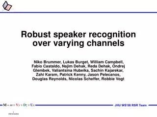
Robust speaker recognition over varying channels Niko Brummer, Lukas Burget,William Campbell, Fabio Castaldo, Najim Dehak, Reda Dehak, Ondrej Glembek, ValiantsinaHubeika, Sachin Kajarekar, Zahi Karam, Patrick Kenny, Jason Pelecanos, Douglas Reynolds, Nicolas Scheffer, Robbie Vogt
Variability refers to changes in channel effects between training and successive detection attempts Channel/session variability encompasses several factors The microphones Carbon-button, electret, hands-free, array, etc The acoustic environment Office, car, airport, etc. The transmission channel Landline, cellular, VoIP, etc. The differences in speaker voice Aging, mood, spoken language, etc. Intersession Variability NIST SRE2008 - Interview speech Different microphone in training and test about 3% EER The same microphone in training and test < 1% EER The largest challenge to practical use of speaker detection systems is channel/session variability
u2 u1 d11 v2 d22 d33 v1 Tools to fight unwanted variability Joint Factor Analysis M = m +Vy +Dz +Ux
Baseline System NIST SRE08 short2-short3 Telephone Speech in Training and Test Miss Probability System based on Joint Factor Analysis False Alarm Probability
SRE NIST Evaluations • Annual NIST evaluations of speaker verification technology (since 1995) using a common paradigm for comparing technologies • All the team members participated in recent 2008 NIST evaluations • JHU workshop provided a great opportunity to: • do common post-evaluation analysis of our systems • combine and improve techniques developed by individual sites • Thanks to NIST evaluations we have: • identified some of the current problems that we worked on • well defined setup and evaluation framework • baseline systems that were trying to extend and improve during the workshop
Subgroups • Diarization using JFA • Factor Analysis Conditioning • SVM – JFA and fast scoring • Discriminative System Optimization
Diarization using JFA Problem Statement • Diarization is an important upstream process for real-world multi-speaker speech • At one level diarization depends on accurate speaker discrimination for change detection and clustering • JFA and Bayesian methods have the promise of providing improvements to speaker diarization Goals • Apply diarization systems to summed telephone speech and interview microphone speech • Baseline segmentation-agglomerative clustering • Streaming system using speaker factors features • New variational-bayes approach using eigenvoices • Measure performance in terms of DER and effect on speaker detection
Factor Analysis Conditioning Problem Statement • A single FA model is sub-optimal across different conditions • Eg.: different durations, phonetic content and recording scenario Goals • Explore two approaches: • - Build FA models specific to each condition and robustly combine multiple models • - Extend the FA model to explicitly model the condition as another source of variability
SVM - JFA Problem Statement The Support Vector Machine is a discriminative recognizer which has proved to be useful for SRE Parameters of generative GMM speaker models are used as features for linear SVM ( sequence kernels) We know Joint Factor Analysis provides higher quality GMMs, but using these as is in SVMs has not been so successful. Goals Analysis of the problem Redefinition of SVM kernels based on JFA? Application of JFA vectors to recently proposed and closely related bilinear scoring techniques which do not use SVMs
Discriminative System Optimization Problem Statement • Discriminative training has proved very useful in speech and language recognition, but has not been investigated in depth for speaker recognition • In both speech and language recognition, the classes (phones, languages) are modeled with generative models, which can be trained with copious quantities of data • But in speaker recognition, our speaker GMMs have at best a few minutes of training typically of only one recording of the speaker Goals • Reformulate the speaker recognition problem as binary discrimination between pairs of recordings which can be (i) of the same speaker, or (ii) of two different speakers • We now have lots of training data for these two classes and we can afford to train complex discriminative recognizers
Relevance MAP adaptation Target speaker model Test data UBM • 2D features • Single Gaussian model • Only mean vector(s) are adapted
Intersession variability Target speaker model UBM High speaker variability High inter-session variability
Intersession variability Target speaker model Test data Decision boundary UBM High speaker variability High inter-session variability
Intersession compensation Target speaker model Test data UBM High speaker variability High inter-session variability For recognition, move both models along the high inter-session variability direction(s) to fit well the test data (e.g. in ML sense)
Probabilistic model proposed by Patrick Kenny Speaker model represented by mean supervector M = m + Vy + Dz + Ux U– subspace with high intersession/channel variability (eigenchannels) V– subspace with high speaker variability (eigenvoices) D - diagonal matrix describing remaining speaker variability not covered by V Gaussian priors assumed for speaker factors y, z and channel factors x Joint Factor Analysis model u2 u1 d11 v2 3D space of model parameters (e.g. 3 component GMM; 1D features) d22 m d33 v1
Working with JFA • Enrolling speaker model: • Given enrollment data and the hyperparameters m,Σ, V, Dand U, obtain MAP point estimates (or posterior distributions) of all factors x, y,z • Most of the speaker information is in low dimensional vector y; less in high dimensional vector z; x should contain only channel related info. • Test: • Given fixed (distributions of) speaker dependent factors y and z, obtain new estimates of channel factors x for test data • Score for test utterance is log likelihood ratio between UBM and speaker model defined by factors x, y, z • Training hyperparameters • Hyperparameters m,Σ, V, Dand U can be estimated from training data using EM algorithm • Posterior distributions of “hidden” factors x, y,z and hyperparameters are alternately estimated to maximize likelihood of training data • Distributions of speaker factors y,z are constraint to be the same for all segments of the same speaker while channel factors x may be different for every segment. u2 u1 d11 v2 d22 m d33 v1
Flavors of JFA • Relevance MAP adaptation • M = m + Dz with D2 = Σ/ τ • where Σ is matrix with UBM variance supervector in diagonal • Eigenchannel adaptation (SDV, BUT) • Relevance MAP for enrolling speaker model • Adapt speaker model to test utterance using U estimated by PCA • JFA without V,with D2 = Σ/ τ(QUT, LIA) • JFA without V,with D trained from data (CRIM) • can be seen as training different τ for each supervector coefficient • Effective relevance factor τef= trace(Σ)/trace(D2) • JFA with V(CRIM) u2 u1 d11 v2 d22 m d33 v1
Flavors of JFA SRE 2006 (all trials, det1) No JFA Eigenchannel adapt. JFA: d2 = Σ/ τ JFA: d trained on data JFA with eigenvoices Full JFA significantly outperform the other JFA configurations.
Subgroups • Diarization based on JFA • Factor Analysis Conditioning • SVM – JFA and fast scoring • Discriminative System Optimization
Diarization Group Douglas Reynolds, Patrick Kenny, Fabio Castaldo, Ciprian Costin
Roadmap • Introduction • Problem definition • Experiment setup • Diarization Systems • Variational Bayes System • Streaming and Hybrid Systems • Analysis and Conclusions
Diarization Segmentation and Clustering • Determine when speaker change has occurred in speech signal (segmentation) • Group together speech segments from same speaker (clustering) • Prior speaker information may or may not be available Where are speaker changes? Which segments are from the same speaker? Speaker A Speaker B
Diarization Applications • Diarization is used as a pre-process for other downstream applications • Human consumption • Annotate transcript with speaker changes/labels • Provide overview of speaker activity • Algorithm consumption • Adaptation of speech recognition system • Application to speaker detection with multi-speaker speech MAX 1sp detector Speaker Diarization Utterance score 1sp detector
Diarization Error Measures • Direct Measure – Diarization Error Rate (DER) • Optimal alignment of reference and hypothesized diarizations • Error is sum of • miss (speaker in reference but not in hypothesis) • false alarm (speaker in hypothesis but not in reference) • speaker-error (mapped reference speaker is not the same as the hypothesized speaker) • Time weighted measure • Emphasizes talkative speakers • Consumer Measure – Effect on speaker detection system • Determine speaker detection error rate when using different diarization output • Focus on NIST SRE 2008 data with a fixed detection system (JFA GMM-UBM system)
Diarization Experiment Data • Summed channels telephone speech • Use summed channel data for test only • (avoid complication of extra clustering in training) • We can derive reference for DER scoring using ASR transcripts from separate channels • (no-score for silence and speaker overlap) • Compare use of diarization to two extremes • Best case: use reference diarization • Worst case: no diarization • Interview microphone speech • Single microphone recording capturing both interviewee (target) and interviewer • Avoid use of unrealistic side information about location of interviewee speech provided in NIST eval • Reference for DER scoring from lavaliere microphones ASR transcripts
Roadmap • Introduction • Problem definition • Experiment setup • Diarization Systems • Variational Bayes System • Streaming and Hybrid Systems • Analysis and Conclusions
Baseline System • Three stages in baseline system • BIC based speaker change detection • Full covariance agglomerative clustering with BIC stopping criterion • Iterative re-segmentation with GMM Viterbi decoding Speaker Change Detection Agglomerative Clustering Initial speaker data Viterbi Decode Train GMMs Final Diarization Refined speaker data
Factor Analysis Applied to Diarization • State of the art speaker recognition systems use hundreds of speaker and channel factors • Processing requires entire utterances – can't be implemented incrementally • State of the art diarization systems require lots of local decisions • Very short (~1 sec) speech segments • Speaker segmentation: is this frame a speaker change point? • Agglomerative clustering: Given two short segments, is the speaker the same? • Proposed solution: Variational Bayes (VB) • Fabio Valente, Variational Bayesian Methods for Audio Indexing, PhD Dissertation, Eurecom, 2005
Advantages of a Bayesian Approach • EM-like convergence guarantees • No premature hard decisions as in agglomerative clustering • This suggested a `soft clustering' heuristic which reduced the diarization error rate of the baseline system by almost 50% • In theory at least, Bayesian methods are not subject to the over-fitting which maximum likelihood methods are prone to • Bayesian model selection is a quantitative version of Occam's razor (David MacKay) • It ought to be possible to determine the number of speakers in a file without resorting to BIC like fudge factors (Fabio Valente)
Eigenvoice Speaker Model • For diarization we use only the eigenvoice component of factor analysis • A supervector s is the concatenation of the mean vectors in a speaker dependent Gaussian mixture model • The supervector m is speaker independent • The matrix V is of low rank • The columns of V are the eigenvoices • The entries of y are the speaker factors • A highly informative prior on speaker dependent GMM's • Adding eigenchannels doesn't help in diarization (so far)
Variational Bayes Diarization • Assume 2 speakers and uniformly segment the file into 1 second intervals • This restriction can be removed in a second pass • Alternate between estimating two types of posterior distribution until convergence • Segment posteriors (soft clustering) • Speaker posteriors (location of the speakers in the space of speaker factors) • Construct GMM's for each speaker and re-segment the data • Iterate as needed
Variational Bayes DiarizationDetails • Begin • Extract Baum-Welch statistics from each segment • On each iteration • For each speaker: • Synthesize Baum Welch statistics by weighting the Baum Welch statistics for each segment by the corresponding posterior • Update the posterior distribution of the speaker factors • For each segment • Update the segment posteriors for each speaker • End • Construct GMM's for each speaker • Re-segment the data • Iterate
Experiment Configuration • Features used for Variational Bayes • 39 dimensional feature set optimized by Brno for speaker recognition • Cepstral coefficients c0, .., c12 + first, second and third order derivatives + Gaussianization + HLDA • Features used in the baseline system and in the re-segmentation phase of Variational Bayes • Un-normalized cepstral coefficients c0, .., c12 • Including c0 was a lucky bug • Factor analysis configuration for Variational Bayes • Universal background model with 512 Gaussians • 200 speaker factors, no channel factors • V matrix scaled by 0.6 • Test set: the summed channel telephone data provided by NIST in the 2008 speaker recognition evaluation • 2215 files, (~200 hours) • NIST Diarization Error used to measure performance • Ground truth diarization is available
Experiment ResultsNIST 2008 Summed Channel Telephone Speech • VB = Variational Bayes • BW = Baum -Welch training of speaker GMM's • Viterbi = re-segmentation with speaker GMM's • The second pass in VB uses a non-uniform segmentation provided by the first pass • Compared to the baseline, soft clustering achieves a 50% reduction in error rates
Roadmap • Introduction • Problem definition • Experiment setup • Diarization Systems • Variational Bayes System • Streaming and Hybrid Systems • Analysis and Conclusions
Streaming SystemLPT Diarization System* Main Ideas Use eigenvoice model for creating a stream of speaker factors Yt computed on a sliding windows Perform segmentation and clustering with these new features Eigenvoice Model: * Based on Castaldo, F.; Colibro, D.; Dalmasso, E.; Laface, P.; Vair, C.,Stream-based speaker segmentation using speaker factors and eigenvoices, ICASSP 2008
Streaming System Feature Extraction Audio Slices Streaming Factor Analysis x1 x2 x3 x4 x5 x6 x7 x8 x9 GMM 1 GMM 2 GMM 1 GMM 2 GMM 1 GMM 2 Slice Clustering
Streaming SystemStream Factor Analysis Y1 Slices Feature Extraction x1 x2 x3 x4 x5 x6 x7 x8 x9 x10 x11 x12 Y2 Viterbi Segmentation Clustering GMM 1 Creating GMMs GMM 2
Streaming SystemStream Factor Analysis First 2 dimensions of y stream
Streaming SystemSlice Clustering A GMM model for each slice is created Last step: clustering the GMMs created in each slice The system decides whether GMMs come from the same or different speakers by using an approximation of the Kullback-Leibler divergence between GMMs Large KL-divergence => new speaker New 60s slice <λ Adapt model GMM 1 Min KL Divergence GMM 2 New GMM Creating new model GMM 3 >λ
Hybrid Clustering Speaker factors works in the streaming diarization system Experiments done during the workshop showed cosine distance between speaker factors produces low speaker detection errors Modifying the baseline system using these new ideas Hybrid Clustering Replace the classical clustering using speaker factors and cosine distance
Hybrid ClusteringDifferent Approaches First Approach: Level Cutting Stop the agglomerative clustering at a certain level and compute speaker factors for each cluster Merge the clusters that have the maximum similarity with respect to the cosine distance Iterate until only two clusters remain Second Approach: Tree Searching Build agglomerative clustering up to the top level Select the nodes that have a number of frames above a threshold Merge the clusters that have the maximum similarity with respect to the cosine distance Iterate until only two clusters remain
Hybrid Clustering Level Cutting S P E A K E R F A C T O R C L U S T E R I N G Y1 Y2 Y1 Y2 Y3 Y1 Y2 Y3 Y4 Y1 Y2 Y3 Y4 Y5 A C G L G U L S O T M E E R R I A N T G I V E 1 2 3 4 5 1 2 3 4 5 6
Hybrid ClusteringTree Searching Threshold=100 180 550 =selected cluster(Y) 110 70 550 70 210 340 110 50 60 70 210 340
Roadmap • Introduction • Problem definition • Experiment setup • Diarization Systems • Variational Bayes System • Streaming and Hybrid Systems • Analysis and Conclusions
DER vs EERSummed Telephone Speech • Some correlation of DER to EER • Systems with DER <10% have comparable EERs • No clear knee in the curve • Still have EER gains (over doing nothing) with relatively poor DER=20% system