Speaker Recognition
Speaker Recognition. Tomi Kinnunen Department of Computer Science University of Joensuu. Lappeenranta, 25.11.2003 ADVANCED TOPICS IN INFORMATION PROCESSING 1. Outline of the Presentation. I Introduction II Speech Production III Feature Extraction IV Speaker Modeling and Matching

Speaker Recognition
E N D
Presentation Transcript
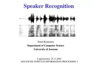
Speaker Recognition Tomi Kinnunen Department of Computer Science University of Joensuu Lappeenranta, 25.11.2003 ADVANCED TOPICS IN INFORMATION PROCESSING 1
Outline of the Presentation I Introduction II Speech Production III Feature Extraction IV Speaker Modeling and Matching V Decision Making VI Error Sources VII Conclusion
Applications • Person authentication • Forensics • Speech recognition • Audio segmentation • Personalized user interfaces
Speech as a Biometric Why speech ? Why not speech ? • The most natural way of communicating • Non-intrusive as a biometric • No special equipment needed • Easy to integrate with other biometrics (multimodal systems) • Not accurate • Can be imitated or resynthesized • Depends on the speaker’s physical and emotional state • Recognition in noisy environments is demanding
Types of Speaker Recognition • Auditive (naive) speaker recognition • By listening to voice samples • Semi-automatic speaker recognition • A human expert locates linguistically comparable speech segments using visual (spectrogram, waveform, …) and auditive cues • Automatic speaker recognition • Only computer involved in the recognition process
“Voiceprint”1 Identification (“Hyvää päivää” spoken by five different male speakers) This is very misleading term (however used in daily media/movies) 1 Who is this?
Intra-Speaker Variability(“Puhujantunnistus” produced by the same male speaker)
Definitions “Please read the following: ‘Vaka vanha väinämöinen’ ” • Speaker identification(1:N matching) • Given a voice sample X and a database of N known speakers • - Who matches X best? (closed-set task) • - Does X match anyone enough close? (open-set task) • Speaker verification(1:1 matching) • Given a voice sample and an identity claim. Is • the speaker who he/she claims to be? • Note: verification is a special case of open-set • identification task with N =1 • Text-dependent recognition • The utterance is known beforehand • (e.g. text-prompted speaker verification) • Text-independent recognition • No assumptions about the utterance
Speech input Training Speaker modeling mode Speaker Feature model extraction database Pattern matching Recognition mode Identity claim Decision logic (verification only) Decision Components of Speaker Recognizer 1.Feature extraction: transformation of the raw speech signal in a compact but effective representation 2. Speaker modeling: training a statistical model of the speaker’s vocal space based on his/her training data (feature vectors) 3. Pattern matching: computing match score between the unknown speaker’s feature vectors and the known speaker(s) models 4. Decision logic: making the decision based on the match score(s)
Speech input Training Speaker modeling mode Speaker Feature model extraction database Pattern matching Recognition mode Identity claim (verification only) Decision Decision logic Part II: Speech Production
3. Vocal tract 2. Larynx 1. Subglottal respiratory system Speech Production Organs
Larynx (1) • Larynx is responsible for different phonation modes(voiceless, voiced, whisper) • During voiceless phonation (e.g. [s] in “star”) and whisper, vocal cords are apart from each other, and the airstream passes through the open glottis (the opening between the vocal cords) • In voiced phonation (e.g. [a] in “star”), vocal folds are successively opening and closing, creating a periodic waveform. The frequency of vibration is called fundamental frequency(or pitch) and abbreviated F0.
Larynx (2) • Average F0 values for male, female, and children are about 120, 220 and 330 Hz • The shape of the glottal pulse is individual, and it is an important determinant of the perceived voice quality (“She has a harsh / rough / breathy / clear /.. voice”)
Vocal Tract (1) • Includes pharyngeal, oral and nasal cavities. The volumes and shapes of these are individual. • Can be roughly characterized by its (time-varying) resonance frequencies called formants
(2n - 1) c Fn = nth formant freq. [Hz] Fn = L = length of the tube [m] 4L • Example: Case N = 1 (neutral vowel [ ] configuration) : e Vocal Tract (2) • Can be modeled as a hard-walled lossless tube resonatorconsisting of N tubes with different cross-sectional areas c= speed of sound in air [m/s]
S(z) = U(z)H(z) s[n] = u[n] * h[n] Frequency domain Time domain Source Filter Source and filter combined Source-Filter Model • The resulting speech spectrum S(z) is a combination of the source spectrum U(z) and the vocal tract transfer function H(z):
Part III: Feature Extraction Speech input Training Speaker modeling mode Speaker Feature model extraction database Pattern matching Recognition mode Identity claim (verification only) Decision Decision logic
Feature Extraction • Raw speech waveform carries too much redundant information • Feature extraction (FE) transforms the original signal into a more compact, stable and discriminative representation • Curse of dimensionality: the number of needed training samples grows exponentially with the dimensionality Speaker modeling is easier in low-dimensional space • Formally, FE is a transformation f : NM, where M << N • Although general-purpose FE methods exist (PCA, LDA, neural networks, ...), domain knowledge (acoustic/phonetics) is necessary
What Is a Good Feature? • Optimal feature has the following properties: (1) High inter-speaker variation (2) Low intra-speaker variation (3) Easy to measure (4) Robust against disguise and mimicry (5) Robust against distortion and noise (6) Maximally independent of the other features • Not a single feature has all these properties ! • For example, F-ratio can be used to measure the discrimination power of a single feature (requirements (1) and (2)) : Variance of speaker means of feature i Average intra-speaker variance of feature i Fi=
Learned, behavioral, functional Phone/word co-occurence patterns, pronounciation modeling, ... • + Robust against channel effect and noise • - Hard to automatically extract • - Requires a lot of training data • - Complicated models • - Text-dependence Lexical and syntactic features Pitch and intensity contours, prosodic dynamics, timing, microprosody, ... Prosodic features Spectrum of phonemes, LTAS, voice quality, formant frequencies, formant bandwidths, ... Phonetic features + Easy to automatically extract + Small amount of data necessary + Easy to model + Text-independence - Easily corrupted by noise and inter-session variability Low-level acoustic features Subband processing, cepstrum, LPC features, PLP, spectral dynamics, modulation spectrum, ... Physiological, organic Features for Speaker Recognition
Frame 2 Frame 1 Frame 3 Frame i ... ... Frame overlap Spectral analysis Window function Frame length Feature vector xi Feature extraction Low-Level Acoustic Feature Extraction • Signal is processed in short frames that are overlapping with each other • From each frame, a feature vector is computed • Typical frame length ~ 20-40 msec, overlapping ~ 30-75 % • Usually frame length is fixed, which is simple to implement • Fixed length does not take into account natural phone length variation and coarticulation effects. Some alternative processing methods include: Pitch-syncronous analysis, variable frame rate analysis (VFR), temporal decomposition (TD)
General Steps Before Feature Extraction • 1. Pre-emphasis filtering : • The natural attenuation that arises from voice source is about -12 dB/octave. Pre-emphasis makes higher frequencies of voiced sounds more apparent • Usually: H(z) = 1 - z-1 , with 1 • 2. Windowing : • Discrete Fourier transform (DFT) assumes that the signal is periodic. Windowing reduces the effect of the spectral artefacts (spectral leakage/smearing) that arise from discontinuities at the frame endpoints. • Typically Hammingwindow is used.
Often static and dynamic features are augmented into a one feature vector Some Commonly Used Features • 1.Static features (local spectrum) • Computed from one frame, gives a “snapshot” of the associated articulators at that time instant • Some commonly used features include: • - Subband processing • - Cepstrum and its variants (mel-cepstrum, LPC-cepstrum) • - LPC-derived features: LSF, LAR, reflection coefficients, … • - F0, log(F0) • 2. Dynamic features (time trajectories of static parameters) • Computed from a few adjacent (e.g. ± 2) frames • Assumed to correlate with speaking rate, coarticulation, rhythm, etc. • The most commonly used parameters are delta- and delta-delta features (1st and 2nd order derivative estimates of any feature)
Frame of speech |FFT| DCT Mel-filtered spectrum Liftering Example: Mel-Frequency Cepstral Coefficients (MFCC) Windowed frame Pre-emphasis + windowing Mel-spaced filter bank Magnitude spectrum Mel-frequency filtering log ( . ) MFCC vector
Part IV: Speaker Modeling and Matching Speech input Training Speaker modeling mode Speaker Feature model extraction database Pattern matching Recognition mode Identity claim (verification only) Decision Decision logic
Speaker Modeling • Given training feature vectors X = {x1, … , xN} produced by speaker i, thetask is to create a statistical model Mi that describes the distribution of the feature vectors • The model should be able to generalize beyond the training samples such that in the recognition stage, unseen vectors are classified correctly • Design of the training material is important! Training material should be phonetically balanced so that it contains instances of all possible phonemes of the language in different contexts • In text-independent recognition, models can be roughly divided into two classes: • Non-parametric models (template models) • Parametric models (stochastic models)
Example of Modeling of 2-d Data Vector quantization (VQ) Gaussian Mixture Model (GMM)
VQ and GMM Speaker Models 1. VQ : [Soong & al., 1987] • Original training set Xis replaced by a smaller set of vectors, called a codebook and denoted here by C • The codebook is formed by clustering the training data by any clustering algorithm (K-means, Split, PNN, SOM, GA, …) • A large codebook represents the original data well, but might overfit to the training vectors (poor generalization) • Typical codebook size in speaker recognition ~ 64..512 2. GMM : [Reynolds and Rose, 1995] • A model consists of K multivariate Gaussian distributions. The component parameters are their a priori probabilities Pi , mean vectors iand covariance matrices i • The parameters (Pi , i , i) are estimated from the training data by maximum likelihood estimation using Expectation Maximization (EM) algorithm • Model size usually less than in VQ (the model itself is more complex) • Considered as state-of-the-art speaker modeling technique
VQ-Based Matching N 1 min ||xi - cj ||2 D(X, C) = j X i=1 • Notation: X = {x1, … , xN} feature vectors of the unknown speaker C = {c1, … , cK} codebook • Define averagequantization distortion as: • The smaller D(X,C) is, the more X and C match each other • Notice that D is not symmetrical: D(X, C) D(C, X )
Notation: • X = {x1, … , xN} feature vectors of the unknown speaker • = {1, … , K}, where j = (Pj , j , j), GMM parameters • The density function of the model is given by: K p(xi | ) = Pj N(xi |j), j=1 where N(xi |j) is the multivariate Gaussian density: N(xi |j) = (2)-d/4|j|-1/2 exp{-1/2 (xi - j)T j-1(xi - j)} • Assuming independent observations, the log likelihood of X with respect to model is given by N P(X | ) = logp(xi | ) i=1 • The larger the log likelihood is, the better X and match each other GMM-Based Matching
”Good” vectors for speaker #2 ”Good” vectors for speaker #1 ”Bad” vectors N 1 wi min ||xi - cj ||2 D(X, C) = j X i=1 Weighted VQ-Matching[Kinnunen and Fränti, 2001; Kinnunen and Kärkkäinen, 2002] • Assign a discriminative weight to code vectors and/or to test sequence vectors
Part V: Decision Making Speech input Training Speaker modeling mode Speaker Feature model extraction database Pattern matching Recognition mode Identity claim Decision logic (verification only) Decision
Decision Making • Let score(X, Si) be the match score between feature vector set X and a speaker model Si • Let us assume that larger score means better match • Let S = {S1,…,SN} be the database of known speakers • 1.Closed-set identification task : • Choose speaker i* for which i* = argmaxiscore(X, Si) 2.Verification task: Accept, score(X, Si) i Reject, score(X, Si) < i Decide i = verification threshold 3.Open-set identification task : Speaker i*, i* = argmaxiscore(X, Si) score(X, Si) No one, otherwise Decide
Verification threshold True speaker distribution Clean environment (training) Impostor distribution Count Score Rejection region Acceptance region True speaker distribution Noisy environment (recognition) Impostor distribution Count Everyone is accepted ! Score Score Normalization (1) • The verification thresholds i are typically determined a posteriori when all speaker scores are available • However, recognition conditions might be different from the training conditions features are different match scores are different the threshold determined from the training data do not make sense anymore
Score Normalization (2) • Purpose of score normalization is to normalize the match scores according to other speakers’ match scores so that relative differences between speaker are transformed similarly in the new environment • One possible normalization is: score’(X, Si) = score(X, Si) - maxjRef{score(X, Sj)} • The reference set Ref contains antispeakers (impostors) of the claimed speaker, and it is called cohort set of speaker i. • There are several methods for choosing the cohort speakers and the size of the cohort. Most common is probably selecting a few (1-10) closest impostors to the claimant speaker
Acoustic environment Transmission path Environmental (additive) noise Channel (convolutive) noise Noisy speech Recording & transmission • Handset / microphone distortions • Recording device interference • Bandlimiting, A/D quantization noise • Speech coding • Background noise • Environment acoustics • Echoing Error Sources • Mismatched acoustic conditionsis the most serious error source. Mismatch can arise from the speaker him/herself, and from the technical conditions • Intra-speaker variability: healthy/ill, sober/drunked, aging, unbalanced speech material, voice disguise, ... • Technical error sources:
Conclusion : Speaker recognition is a challenging and very multidisclipinary research topic
References [Kinnunen and Fränti, 2001] T. Kinnunen and P. Fränti, “Speaker Discriminative Weighting Method for VQ- Based Speaker Identification,” Proc. Audio- and Video-Based Biometric Person Authentication(AVBPA 2001), pp. 150-156, Halmstad, Sweden, 2001. [Kinnunen and Kärkkäinen, 2002] T. Kinnunen and I. Kärkkäinen, “Class-Discriminative Weighted Distortion Measure for VQ-Based Speaker Identification,” Proc. Joint IAPR Int.Workshop on Stat. Pattern Recognition (S+SPR2002), pp. 681-688, Windsor, Canada, 2002. [Reynolds and Rose, 1995] D.A. Reynolds and R.C. Rose, “Robust Text-Independent Speaker Identification Using Gaussian Mixture Speaker Models,” IEEE Trans. Speech & Audio Processing, 3(1), pp. 72-83, 1995. [Soong & al., 1987] F.K. Soong and A.E. Rosenberg A.E. and B.-H. Juang and L.R. Rabiner, “A Vector Quantization Approach to Speaker Recognition,” AT & T Technical Journal, vol. 66, pp. 14-26, 1987. Main scientific journals :IEEE Trans. Speech and Audio Processing, Speech Communications, Journal of the Acoustic Society of America, Digital Signal Processing, Pattern Recognition Letters, Pattern Recognition Main conferences :Int. Conference on Acoustics, Speech and Signal Processing (ICASSP), Eurospeech, Int. Conference on Spoken Language Processing (ICSLP) http://cs.joensuu.fi/pages/pums/index.html See also: http://cs.joensuu.fi/pages/tkinnu/research/index.html