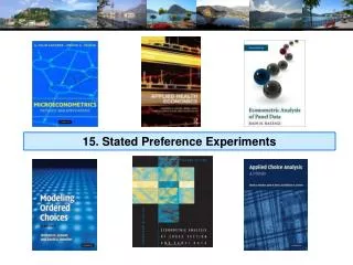
15. Stated Preference Experiments
15. Stated Preference Experiments. Panel Data. Repeated Choice Situations Typically RP/SP constructions (experimental) Accommodating “panel data” Multinomial Probit [Marginal, impractical] Latent Class Mixed Logit. Application: Shoe Brand Choice. S imulated Data: Stated Choice,

15. Stated Preference Experiments
E N D
Presentation Transcript
Panel Data • Repeated Choice Situations • Typically RP/SP constructions (experimental) • Accommodating “panel data” • Multinomial Probit [Marginal, impractical] • Latent Class • Mixed Logit
Application: Shoe Brand Choice • Simulated Data: Stated Choice, • 400 respondents, • 8 choice situations, 3,200 observations • 3 choice/attributes + NONE • Fashion = High / Low • Quality = High / Low • Price = 25/50/75,100 coded 1,2,3,4 • Heterogeneity: Sex (Male=1), Age (<25, 25-39, 40+) • Underlying data generated by a 3 class latent class process (100, 200, 100 in classes)
Stated Choice Experiment: Unlabeled Alternatives, One Observation t=1 t=2 t=3 t=4 t=5 t=6 t=7 t=8
Customers’ Choice of Energy Supplier • California, Stated Preference Survey • 361 customers presented with 8-12 choice situations • Supplier attributes: • Fixed price: cents per kWh • Length of contract • Local utility • Well-known company • Time-of-day rates (11¢ in day, 5¢ at night) • Seasonal rates (10¢ in summer, 8¢ in winter, 6¢ in spring/fall)
Revealed and Stated Preference Data • Pure RP Data • Market (ex-post, e.g., supermarket scanner data) • Individual observations • Pure SP Data • Contingent valuation • Combined (Enriched) RP/SP • Mixed data • Expanded choice sets
Customers’ Choice of Energy Supplier • California, Stated Preference Survey • 361 customers presented with 8-12 choice situations • Supplier attributes: • Fixed price: cents per kWh • Length of contract • Local utility • Well-known company • Time-of-day rates (11¢ in day, 5¢ at night) • Seasonal rates (10¢ in summer, 8¢ in winter, 6¢ in spring/fall)
Population Parameter Distributions • Normal for: • Contract length • Local utility • Well-known company • Log-normal for: • Time-of-day rates • Seasonal rates • Price coefficient held fixed
Estimated Model Estimate Std error Price -.883 0.050 Contract mean -.213 0.026 std dev .386 0.028 Local mean 2.23 0.127 std dev 1.75 0.137 Known mean 1.59 0.100 std dev .962 0.098 TOD mean* 2.13 0.054 std dev* .411 0.040 Seasonal mean* 2.16 0.051 std dev* .281 0.022 *Parameters of underlying normal. i= exp(mean+sd*wi)
Distribution of Brand Value Brand value of local utility Standard deviation =1.75¢ 10% dislike local utility 0 2.23¢
Time of Day Rates (Customers do not like - lognormal) Time-of-day Rates 0 -10.4 Seasonal Rates -10.2 0
Expected Preferences of Each Customer Customer likes long-term contract, local utility, and non-fixed rates. Local utility can retain and make profit from this customer by offering a long-term contract with time-of-day or seasonal rates.
Choice Strategy • Hensher, D.A., Rose, J. and Greene, W. (2005) The Implications on Willingness to Pay of Respondents Ignoring Specific Attributes (DoD#6) Transportation, 32 (3), 203-222. • Hensher, D.A. and Rose, J.M. (2009) Simplifying Choice through Attribute Preservation or Non-Attendance: Implications for Willingness to Pay, Transportation Research Part E, 45, 583-590. • Rose, J., Hensher, D., Greene, W. and Washington, S. Attribute Exclusion Strategies in Airline Choice: Accounting for Exogenous Information on Decision Maker Processing Strategies in Models of Discrete Choice, Transportmetrica, 2011 • Hensher, D.A. and Greene, W.H. (2010) Non-attendance and dual processing of common-metric attributes in choice analysis: a latent class specification, Empirical Economics 39 (2), 413-426 • Campbell, D., Hensher, D.A. and Scarpa, R. Non-attendance to Attributes in Environmental Choice Analysis: A Latent Class Specification, Journal of Environmental Planning and Management, proofs 14 May 2011. • Hensher, D.A., Rose, J.M. and Greene, W.H. Inferring attribute non-attendance from stated choice data: implications for willingness to pay estimates and a warning for stated choice experiment design, 14 February 2011, Transportation, online 2 June 2001 DOI 10.1007/s11116-011-9347-8.
Individual Explicitly Ignores Attributes • Hensher, D.A., Rose, J. and Greene, W. (2005) The Implications on Willingness to Pay of Respondents Ignoring Specific Attributes (DoD#6) Transportation, 32 (3), 203-222. • Hensher, D.A. and Rose, J.M. (2009) Simplifying Choice through Attribute Preservation or Non-Attendance: Implications for Willingness to Pay, Transportation Research Part E, 45, 583-590. • Rose, J., Hensher, D., Greene, W. and Washington, S. Attribute Exclusion Strategies in Airline Choice: Accounting for Exogenous Information on Decision Maker Processing Strategies in Models of Discrete Choice, Transportmetrica, 2011 Choice situations in which the individual explicitly states that they ignored certain attributes in their decisions.
Stated Choice Experiment Ancillary questions: Did you ignore any of these attributes?
Appropriate Modeling Strategy • Fix ignored attributes at zero? Definitely not! • Zero is an unrealistic value of the attribute (price) • The probability is a function of xij – xil, so the substitution distorts the probabilities • Appropriate model: for that individual, the specific coefficient is zero – consistent with the utility assumption. A person specific, exogenously determined model • Surprisingly simple to implement
Individual Implicitly Ignores Attributes • Hensher, D.A. and Greene, W.H. (2010) Non-attendance and dual processing of common-metric attributes in choice analysis: a latent class specification, Empirical Economics 39 (2), 413-426 • Campbell, D., Hensher, D.A. and Scarpa, R. Non-attendance to Attributes in Environmental Choice Analysis: A Latent Class Specification, Journal of Environmental Planning and Management, proofs 14 May 2011. • Hensher, D.A., Rose, J.M. and Greene, W.H. Inferring attribute non-attendance from stated choice data: implications for willingness to pay estimates and a warning for stated choice experiment design, 14 February 2011, Transportation, online 2 June 2001 DOI 10.1007/s11116-011-9347-8.
Stated Choice Experiment Individuals seem to be ignoring attributes. Uncertain to the analyst
The 2K model • The analyst believes some attributes are ignored. There is no indicator. • Classes distinguished by which attributes are ignored • Same model applies, now a latent class. For K attributes there are 2K candidate coefficient vectors
6 attributes implies 64 classes. Strategy to reduce the computational burden on a small sample
Posterior probabilities of membership in the nonattendance class for 6 models
Revealed vs. Stated Preference Data • Advantage: Actual observations on actual behavior • Disadvantage: Limited range of choice sets and attributes – does not allow analysis of switching behavior.
Application Survey sample of 2,688 trips, 2 or 4 choices per situation Sample consists of 672 individuals Choice based sample Revealed/Stated choice experiment: Revealed: Drive,ShortRail,Bus,Train Hypothetical: Drive,ShortRail,Bus,Train,LightRail,ExpressBus Attributes: Cost –Fuel or fare Transit time Parking cost Access and Egress time
Mixed Logit Approaches • Pivot SP choices around an RP outcome. • Scaling is handled directly in the model • Continuity across choice situations is handled by random elements of the choice structure that are constant through time • Preference weights – coefficients • Scaling parameters • Variances of random parameters • Overall scaling of utility functions
Pooling RP and SP Data Sets • Enrich the attribute set by replicating choices • E.g.: • RP: Bus,Car,Train (actual) • SP: Bus(1),Car(1),Train(1) Bus(2),Car(2),Train(2),… • How to combine?
Each person makes four choices from a choice set that includes either 2 or 4 alternatives. The first choice is the RP between two of the 4 RP alternatives The second-fourth are the SP among four of the 6 SP alternatives. There are 10 alternatives in total. A Stated Choice Experiment with Variable Choice Sets
Enriched Data Set – Vehicle Choice Choosing between Conventional, Electric and LPG/CNG Vehicles in Single-Vehicle Households David A. Hensher William H. Greene Institute of Transport Studies Department of Economics School of Business Stern School of Business The University of Sydney New York University NSW 2006 Australia New York USA September 2000
Fuel Types Study • Conventional, Electric, Alternative • 1,400 Sydney Households • Automobile choice survey • RP + 3 SP fuel classes

