Download
1 / 47
470 likes | 560 Views
Explore solar-friendly architectural thinking with computer program ArchiPlan for energy-efficient building layouts. Evaluate layouts based on compactness, construction requirements, and energy effectiveness. Estimate energy losses and gains to optimize solar utilization. Quick analysis of solar beam and diffuse radiation for complex architectural designs.

E N D
Estimation of solar radiation for buildings with complexarchitectural layouts Arch. Stoyanka Ivanova University of Architecture, Civil Engineering and Geodesy Sofia, Bulgaria
If we want the “solar friendly” architectural thinking to be accepted widely, then we have to think how it could be applied still in the beginning of the architectural creative process – when the idea of the building is shaped and especially in the process of creating of the architectural layout. It’s possible to use a computer program not only to draw a desired layout, but also to create it. It’s hard to simulate the architectural creative process, but with the increase of the present computer might this is not already a “mission impossible”. 1 Introduction
The program ArchiPlan is created to assist the architect in the process of searching of initial architectural idea – architectural layout. The program generates hundreds of 2D orthogonal architectural layouts for just few seconds. 1 Introduction
In the beginning the architect describes the elements (rooms) of the desired layout: names of rooms square surface of each room functional relations between rooms requirements for each element for exposure desired grid, etc. 1 Introduction
1 Introduction Example (15 rooms)
1 Introduction Matrix of functional relations between rooms
1 Introduction With these data the program ArchiPlan generates 602 architectural layouts for less than 4 seconds…
1 Introduction Exemplary architectural layouts, generated by the program ArchiPlan:
1 Introduction • These layouts have to be evaluated, so the program can offer the architect only the best of them. The program uses the following criteria to rank all generated layouts: • compactness (as a planning quality) • construction’s requirements • energy effectiveness (energy gains and losses) • The weight of these three criteria could vary, regarding the architect’s final goal.
1 Introduction The program ArchiPlan sorts the generated architectural layouts on compactness… Let’s see worst 5 and top 10 layouts…
2 Methodology The energy effectiveness of an architectural layout has two sides – energy losses and energygains. In this too early moment of the architectural process the energy losses could be evaluated with the compactness of the building - the surface-area-to-volume ratio - a proportion between the total exterior surface and internal volume. As less is this number, as more compact is the building and lower the energy losses.
2 Methodology • Since June 30th a new calculation of supposed energy losses was added to the program. It uses a difference between inside and outside air temperature and supposed heat transmission coefficient. • The energy effectiveness is calculated as follows:
2 Methodology To evaluate energy gains, the program ArchiPlan estimates the quantity of incoming solar energy [Wh] to the building outside surface (exterior walls and roof) for the whole heating season. In this so early stage is convenient to use 2.5D model – with only horizontal and vertical surfaces.
2 Methodology Two methods of solar energy estimationare created. The final goal of the first method is to rank the hundreds of generated architectural layouts considering their energy effectiveness. In this case is important to receive quick results, even with some little inexactness. This is why we need to simplify computation of the summary solar radiation, received by all exterior surfaces.
2 Methodology The second method is created to estimate the solar radiation, received by each particular vertical wall of a layout. The goal is to allow the architect to study how a specific architectural layout can utilize the incoming solar energy in best way. Such information could help him to find the best positions for the wall apertures - windows and glazed doors on the walls of a complex architectural layout.
3.1 Quick analysis of summary beam radiation The exterior surface of our 2.5D model is projected on a plane, normal to solar beam.
3.1 Quick analysis of summary solar beam radiation Area of roof’s projection: Area of walls’ projection: df – front of projection: Beam radiation:
3.2 Quick analysis of summary diffuse radiation For the diffuse radiation RD [W] is valid the formula: • Dic [W.m-2] - the diffuse irradiance on each external surface (walls or roof) of the building • Ai - area of this surface [m2] • Hofierka and Šúri in their work “The solar radiation model for Open source GIS” described how to estimate the diffuse irradiance on horizontal and inclined surfaces, when they are sunlit, potentially sunlit or shadowed. But this model has to be extended for the cases, when one or more near objects with limited size hide parts of the sky, as it is for the buildings with complex architectural layouts.
3.2 Quick analysis of summary diffuse radiation According Hofierka for inclined surfaces in shadow: • Dhc is diffuse irradiance on a horizontal surface • F(γN) is a function, which convert the diffuse irradiance on a horizontal surface into diffuse irradiance on an inclined surface under anisotropic clear sky: • ri(γN)=(1+cos γN)/ 2 is a fraction of the sky dome, viewed by an inclined surface. • For unobstructedsurfaces in shadow of our 2.5D model, N=0.25227 according Muneer and Hofierka: • when γN=0 (for horizontal surface): F(γN)=1 • when γN=π/2 (for vertical surface): F(γN)=0.356
3.2 Quick analysis of summary diffuse radiation Let’s consider this wall configuration:
3.2 Quick analysis of summary diffuse radiation For the wall A0 a part of the sky is hidden by both other walls. I propose such equation to the mentioned model: • DFi is a function, which transforms the value of the diffuse irradiance on a horizontal surface to a value of diffuse irradiance, incoming from partially shaded anisotropic sky, onto an inclined surface (in our example it’s vertical):
3.2 Quick analysis of summary diffuse radiation • α1 and α2 are azimuths of the furthest ends of the neighbor walls A1 and A2 • C1,2 is a correction coefficient for the visible part of the sky in horizontal direction, between azimuths α1 and α2 • VT1 and VT2 are the correction values due of the spherical triangles T1 and T2 above the walls A1 and A2on the stereographic projection.
3.2 Quick analysis of summary diffuse radiation For estimation of C1,2 this equation is proposed: where α1=arctg(dx1/dy1) and α2=arctg(dx2/dy2). If dy1=0 then α1=-π/2 and VT1=0. If dy2=0 then α2=π/2 and VT2=0. If both dy1and dy2 are 0, then C1,2=1, VT1 and VT2 are 0. In all other cases the values of VT1 or VT2 are greater than 0.
3.2 Quick analysis of summary diffuse radiation In the figure are illustrated the variable x1a and angle β1, which are necessary to estimate the value of VT1. AT1 is the area of segment T1 in the same figure.
3.2 Quick analysis of summary diffuse radiation I propose the following approximate equation of VT1 to take into consideration at least partially the anisotropic nature of the diffuse radiation: The transforming function DFi (corrected F(γN)) has to be used to calculate diffuse radiation also on sunlit or partially shaded surfaces. Within this quick method I estimate Dic only once for the center of each examined vertical wall.
3.3 Quick analysis of solar radiation under real sky • Finally the computation of overcast radiation for inclined surfaces is analogous to theprocedure described for clear-sky model (Hofierka and Šúri), using the modified values of beam and diffuse irradiance because of the concrete values of beam and diffuse components of theclear-sky index (Kbc, Kdc). • The layouts with best energy effectiveness are compact with southerly exposure of the larger dimension of the building and flat south vertical wall. As higher is the percent of diffuse radiation under the real sky, as more important is the compactness.
3.3 Quick analysis of solar radiation under real sky The program ArchiPlan sorts the generated architectural layouts on energy effectiveness… Let’s see worst 5 and top 10 layouts…
4.1 Detailed analysis of beam and diffuse radiation When the rank list of all generated architectural layouts is ready, the architect could examine the best of them, with the help of a detailed analysis of received solar radiation by each vertical wall to find best place for windows and glazed doors on each floor.
4.1.1 Detailed analysis of incoming beam radiation • According detailed methodology in “Solar radiation and shadow modeling with adaptive triangular meshes” byMontero et al: • B0c is the beam irradiance normal to the solar beam • δexp is the solar incidence angle between the sun and an inclined surface • Lf is calculated lighting factor for the concrete wall, day and time (0 – completely shaded wall; 1 - sunlit wall; between 0 and 1 – partially shadowed wall)
4.1.2 Detailed analysis of incoming diffuse radiation The quantity of diffuse radiation for each fragment of each wall is different. So for a detailed analysis each wall is divided in horizontal and vertical directions and the program applies to these small fragments the estimations, described in the previous section.
4.1.2 Detailed analysis of incoming diffuse radiation For this wall configuration: DFi – the value of the diffuse transforming function for the wall with length b and height h, is: • M is number of fragments in horizontal direction • N is number of fragments in vertical direction • dx is size of a fragment in horizontal direction • dz is size of a fragment in vertical direction • (xj, zk) – center of a fragment of this vertical wall
4.1.2 Detailed analysis of incoming diffuse radiation Instead with this double sum, the exact value of diffuse transforming function for the same vertical wallcan be estimated with this double definiteintegral: The value of the integral is:
4.1.2 Detailed analysis of incoming diffuse radiation For different wall configurations the double integral and its result looks also different. There are 4 basic double integrals and many combinations between them for different wall configurations . I still work on some combinations.
4.2 Balance principles of incoming and received diffuse radiation Balance principle 1: The quantity of diffuse radiation, crossed an opening (with area Aopening ), is equal to sum of the quantities of diffuse radiation, received by the surfaces (with areas Ai ), which are behind this opening. From this is easy to come to: • DFopening is value of the diffuse transforming function for the planar surface of the opening • DFi is the value for each receiving surface behind the opening • DFj and Aj are value of the transforming function and area of a small fragment j of the surface i
4.2.1 Balance principle 1 - example Opening EFGH Wall ABFE Wall BCGF Wall CDHG Wall ADHE Base ABCD
4.2.1 Balance principle 1 - example For isotropic sky and AB=2, BC=1, AE=3: 2 = 2 All values of DF are calculated with different combinations of mentioned double integral.
4.2.2 Balance principle 2 of incoming and received diffuse radiation Balance principle 2: The quantity of diffuse radiation, crossed two or more openings (with area Ak ), is equal to sum of the quantities of diffuse radiation, received by the surfaces (with areas Ai ), which are behind each of the openings. From this is easy to come to: • DFk is value of the diffuse transforming function for opening k • DFik is the value for the surface i, generated by the incoming diffuse radiation through opening k. • DF has to be defined twice for the planes of vertical openings - for inside and outside face of examined volume. • The value of the transforming function of the surface i with fragments j, for the incoming diffuse radiation from all openings, is:
4.2.2 Balance principle 2 - example Opening EFGH Opening ABFE Surface ABFE Wall BCGF Wall CDHG Wall ADHE Base ABCD
4.2.2 Balance principle 2 - example For isotropic sky and AB=2, BC=1, AE=3: 5 = 5
4.2.2 Balance principle 2 - example Here is another viewpoint to the same example: Wall BCGF Wall CDHG Wall ADHE Opening ABFE Opening EFGH Here we have 2 interesting equalities: 3 = 3 5 = 5 The summary product of DF and Area for these 3 vertical walls is 3.646776
4.2.2 Balance principle 2 - example This is the main practical advantage from both balance principles. It helps to calculate very easy the summary diffuse radiation on a complex wall configuration. The main part of it (pink values) comes across an endless high vertical opening, so for these values we can simplify the outline of the layout in this way:
5 Discussion • Both equations from the balance principles can be proved for isotropic sky analytically with already mentioned double integrals. It’s really beautiful mathematics, just “music of the projected spheres”. • I wasn’t able to prove both balance rules for anisotropic sky numerically. The proof is not obvious and will be more difficult. It could be possible with better knowledge of sky’s anisotropy. • In spite of this the consequences of the second balance rule can be implemented into calculations for obstructed anisotropic sky and to receive values with good approximation. Under real sky this inexactness will be even more unimportant. • Both balance principles and corresponding equations could also be applied to beam and total radiation, to sunlit or partially shadowed surfaces, and for different sky types.
It’s proposed a numerical model for estimation of the solar radiation on the external vertical walls of a building with complex architectural layout. This could help the architect to think more about the solar gains and to choose the best solar friendly architectural layout. Further research is needed to precise the calculation of the diffuse radiation from anisotropic sky for spherical triangles above the vertical walls. The balance principles and corresponding equations are a good start base for further improvement of this model for both isotropic and anisotropic sky. Calculations of reflected radiation and analysis of solar radiation in summer will be added in the future. 6 Conclusion and future work
Muneer, T., Solar radiation model for Europe. Building services engineering research and technology, 1990, vol. (11) Hofierka, J., Šúri M., The solar radiation model for Open source GIS: implementation and applications, Open source GIS - GRASS users conference, Trento, Italy, 2002 Montero, G. et al, Solar radiation and shadow modeling with adaptive triangular meshes, Sol. Energy, 2009, doi:10.1016/j.solenar.2009.01.004 Thank you! 7 References