Download
1 / 26
260 likes | 495 Views
Explicit Simulations of the Intertropical Convergence Zone. Changhai Liu and Mitchell W. Moncrieff Present by Xiaoyu Liu. Outline. Motivation Model description Assumptions Initial state Simulation Off-equator maximum convection stage Equatorial maximum convection stage

E N D
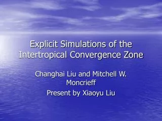
Explicit Simulations of the Intertropical Convergence Zone Changhai Liu and Mitchell W. Moncrieff Present by Xiaoyu Liu
Outline • Motivation • Model description • Assumptions • Initial state • Simulation • Off-equator maximum convection stage • Equatorial maximum convection stage • Formation of the equatorial easterlies • Conclusion and future work • Acknowledgment
Motivation • ITCZ is one of the most important components of the global circulation • What is the physical mechanism regulating the formation and latitude preference of ITCZ? • SST? • Ekman pumping and moisture availability? • Low level convergence? • Cross-equatorial pressure gradients and radiative-convective instability?
Two dimensional Eulerian version of the nonhydrostatic Eulerian/Semi-Lagrangian anelastic model Features: Domain: 16000Km * 24Km Grid: horizontal 5Km; vertical 0.3Km Boundary conditions: Rigid bottom; free-slip top Model Z 16000 km 24 km S.P EQ N.P Y
Assumptions • theta and r equal to average value anytime • Absorbing layer at boundaries • Constant SST 302.5K • Surface moisture and sensible heat flux are given by TOGA COARE surface flux algorithm • Time-independent and horizontal uniform radiative cooling • -1.5K/day below 12km decrease linearly to zero at the top
Initial State • A resting atmosphere • T and q given by average condition of Dec 19-26 1992 in TOGA COARE • Start with small random perturbations of theta and r
Simulation • Period: 100 days • Goal: Statistical quasi-equilibrium • Convective pattern: • Off-equator maximum convection stage • Equatorial maximum convection stage
FIG. 1. Space–time distributions of surface precipitation rate during (a) days 1–25, (b) days 26–50, (c) days 51–75, and (d) days 76–100. The light and dark shading correspond to rainfall intensity greater than 1 and 10 mm h−1, respectively. The equator is located at the center of the domain.
FIG. 2. Spatial distributions of surface precipitation rate averaged over (a) the early 40-day integration and (b) the late 60-day integration. The field is smoothed with a 500-km running mean filter.
FIG. 3. Spatial distributions of cloud amount averaged over (a) the early 40-day integration and (b) the late 60-day integration. The light, moderate dark, and heavy dark shading correspond to cloud fraction greater than 5%, 15%, and 25%, respectively.
Off-equator maximum convection stage FIG. 4a. Physical fields averaged from days 16 to 25. Meridional wind (1 m s−1 contour interval), The white and dark shadings correspond to vertical velocity less than -2.5 * 10−3 m s−1 and greater than 2.5 * 10−3 m s−1, respectively
Off-equator maximum convection stage FIG. 4b. Physical fields averaged from days 16 to 25. zonal wind (2 m s−1 contour interval) The white and dark shadings correspond to vertical velocity less than -2.5 * 10−3 m s−1 and greater than 2.5 *10−3 m s−1, respectively
Off-equator maximum convection stage FIG. 4c. Physical fields averaged from days 16 to 25. temperature perturbation (1-K contour interval)
Off-equator maximum convection stage FIG. 4d. Physical fields averaged from days 16 to 25. water vapor mixing ratio perturbation (0.5 g kg−1 contour interval)
Summary of off-equator maximum convection stage • Vigorous convection is off-equator, rarely occurs near equator • Convection is asymmetric • Equatorward flow at upper levels and poleward flow at lower levels • Deep equatorial easterly wind • Westerly jets
Equatorial maximum convection stage FIG. 5. Evolution of the space-averaged precipitation rate (solid line) and CAPE (dashed line) over a 1500-km-wide area centered at the equator during (a) days 50–75 and (b) days 75–100.
Equatorial maximum convection stage FIG. 6a. Physical fields averaged from days 81 to 90. Meridional wind (1 m s−1 contour interval), The white and dark shadings correspond to vertical velocity less than -2.5 * 10−3 m s−1 and greater than 2.5 * 10−3 m s−1, respectively
Equatorial maximum convection stage FIG. 6b. Physical fields averaged from days 81 to 90. zonal wind (2 m s−1 contour interval) The white and dark shadings correspond to vertical velocity less than −2.5 × 10⁻³ m s−1 and greater than 2.5 × 10⁻³ m s−1, respectively
Equatorial maximum convection stage FIG. 6c. Physical fields averaged from days 81 to 90. temperature perturbation (1-K contour interval)
Equatorial maximum convection stage FIG. 6d. Physical fields averaged from days 81 to 90. water vapor mixing ratio perturbation (0.5 g kg−1 contour interval)
Summary of equatorial maximum convection stage • Single equatorial ITCZ-like morphology • Convection concentrated in a narrow area around the equator and not continuous • Wavelike vertical structure and opposite in sign in two hemispheres • Two-cell vertical structure • Easterly uniformly distributed in vertical • No jet like structure
Formation of the equatorial easterlies FIG. 7a. Evolution of the equatorial easterly wind averaged over a 1000-km-wide area centered at equator for control simulation
Formation of the equatorial easterlies • Zonal momentum equation Coriolis torque Zonal wind tendency Horizontal Mom. Flux convergence Vertical Mom. Flux convergence
Formation of the equatorial easterlies FIG. 8. Evolution of the equatorial zonal wind tendency by (a) horizontal momentum flux convergences, (b) vertical momentum flux convergences, and (c) Coriolis torques averaged over a 1000-km-wide area centered at the equator during days 10–60. Contour interval is 1 m s−1 day−1
Conclusion and future work • Two distinct convective patterns in the Tropics are obtained during the 100-day integration • Off-equator ITCZs • Single ITCZ at the equator • Highly idealized experimental setup and 2-D assumption exclude some features • Future work • 3-D explicit studies
Acknowledgment • Genuine authors Changhai Liu and Mitchell W. Moncrieff • Dr. David Nolan