Download
1 / 76
780 likes | 1.09k Views
2. Chapter. Data Collection. Data Vocabulary Level of Measurement Time Series and Cross-sectional Data Sampling Concepts Sampling Methods Data Sources Survey Research. McGraw-Hill/Irwin. © 2008 The McGraw-Hill Companies, Inc. All rights reserved.

E N D
2 Chapter Data Collection Data Vocabulary Level of Measurement Time Series and Cross-sectional Data Sampling Concepts Sampling Methods Data Sources Survey Research McGraw-Hill/Irwin © 2008 The McGraw-Hill Companies, Inc. All rights reserved.
In scientific research, data arise from experiments whose results are recorded systematically. • In business, data usually arise from accounting transactions or management processes. Data Vocabulary • Data is the plural form of the Latin datum (a “given” fact). • Important decisions may depend on data.
Data Vocabulary • Subjects, Variables, Data Sets • We will refer to Data as plural and data set as a particular collection of data as a whole. • Observation – each data value. • Subject(or individual) – an item for study (e.g., an employee in your company). • Variable – a characteristic about the subject or individual (e.g., employee’s income).
Data Vocabulary • Subjects, Variables, Data Sets • Three types of data sets:
Data Vocabulary • Subjects, Variables, Data Sets Consider the multivariate data set with 5 variables 8 subjects 5 x 8 = 40 observations
Types of Data Attribute(qualitative) Numerical(quantitative) Verbal LabelX = economics(your major) CodedX = 3(i.e., economics) DiscreteX = 2(your siblings) ContinuousX = 3.15(your GPA) Data Vocabulary • Data Types • A data set may have a mixture of data types.
Data Vocabulary • Attribute Data • Also called categorical, nominal or qualitative data. • Values are described by words rather than numbers. • For example, - Automobile style (e.g., X = full, midsize, compact, subcompact).- Mutual fund (e.g., X = load, no-load).
Data Vocabulary • Data Coding • Coding refers to using numbers to represent categories to facilitate statistical analysis. • Coding an attribute as a number does not make the data numerical. • For example, 1 = Bachelor’s, 2 = Master’s, 3 = Doctorate • Rankings may exist, for example, 1 = Liberal, 2 = Moderate, 3 = Conservative
Data Vocabulary • Binary Data • A binary variable has only two values, 1 = presence, 0 = absence of a characteristic of interest (codes themselves are arbitrary). • For example, 1 = employed, 0 = not employed 1 = married, 0 = not married 1 = male, 0 = female 1 = female, 0 = male • The coding itself has no numerical value so binary variables are attribute data.
Data Vocabulary • Numerical Data • Numerical or quantitative data arise from counting or some kind of mathematical operation. • For example, - Number of auto insurance claims filed in March (e.g., X = 114 claims).- Ratio of profit to sales for last quarter (e.g., X = 0.0447). • Can be broken down into two types – discrete or continuous data.
Data Vocabulary • Discrete Data • A numerical variable with a countable number of values that can be represented by an integer (no fractional values). • For example, - Number of Medicaid patients (e.g., X = 2).- Number of takeoffs at O’Hare (e.g., X = 37).
Data Vocabulary • Continuous Data • A numerical variable that can have any value within an interval (e.g., length, weight, time, sales, price/earnings ratios). • Any continuous interval contains infinitely many possible values (e.g., 426 < X < 428).
Level of Measurement • Four levels of measurement for data:
Level of Measurement • Nominal Measurement • Nominal data merely identify a category. • Nominal data are qualitative, attribute, categorical or classification data (e.g., Apple, Compaq, Dell, HP). • Nominal data are usually coded numerically, codes are arbitrary (e.g., 1 = Apple, 2 = Compaq, 3 = Dell, 4 = HP). • Only mathematical operations are counting (e.g., frequencies) and simple statistics.
Level of Measurement • Ordinal Measurement • Ordinal data codes can be ranked(e.g., 1 = Frequently, 2 = Sometimes, 3 = Rarely, 4 = Never). • Distance between codes is not meaningful (e.g., distance between 1 and 2, or between 2 and 3, or between 3 and 4 lacks meaning). • Many useful statistical tests exist for ordinal data. Especially useful in social science, marketing and human resource research.
Level of Measurement • Interval Measurement • Data can not only be ranked, but also have meaningful intervals between scale points (e.g., difference between 60F and 70F is same as difference between 20F and 30F). • Since intervals between numbers represent distances, mathematical operations can be performed (e.g., average). • Zero point of interval scales is arbitrary, so ratios are not meaningful (e.g., 60F is not twice as warm as 30F).
Level of Measurement • Likert Scales • A special case of interval data frequently used in survey research. • The coarseness of a Likert scale refers to the number of scale points (typically 5 or 7).
Level of Measurement • Likert Scales • A neutral midpoint (“Neither Agree Nor Disagree”) is allowed if an odd number of scale points is used or omitted to force the respondent to “lean” one way or the other. • Likert data are coded numerically (e.g., 1 to 5) but any equally spaced values will work.
Level of Measurement • Likert Scales • Careful choice of verbal anchors results in measurable intervals (e.g., the distance from 1 to 2 is “the same” as the interval, say, from 3 to 4). • Ratios are not meaningful (e.g., here 4 is not twice 2). • Many statistical calculations can be performed (e.g., averages, correlations, etc.).
Level of Measurement • Likert Scales • More variants of Likert scales:
Level of Measurement • Ambiguity • Grades are usually coded numerically (A = 4, B = 3, C = 2, D = 1, F = 0) and are used to calculate a mean GPA. • Is the interval from 3.0 to 4.0 really the same as the interval from 1.0 to 2.0? • What is the underlying reality ranging from 0 to 4 that we are measuring? • Best to be conservative and limit statistical tests to those for ordinal data.
Level of Measurement • Ratio Measurement • Ratio data have all properties of nominal, ordinal and interval data types and also possess a meaningful zero (absence of quantity being measured). • Because of this zero point, ratios of data values are meaningful (e.g., $20 million profit is twice as much as $10 million). • Zero does not have to be observable in the data, it is an absolute reference point.
Level of Measurement • Use the following procedure to recognize data types:
Level of Measurement • Changing Data by Recoding • In order to simplify data or when exact data magnitude is of little interest, ratio data can be recoded downward into ordinal or nominal measurements (but not conversely). • For example, recode systolic blood pressure as “normal” (under 130), “elevated” (130 to 140), or “high” (over 140). • The above recoded data are ordinal (ranking is preserved) but intervals are unequal and some information is lost.
We are interested in trends and patterns over time (e.g., annual growth in consumer debit card use from 1999 to 2006). Time Series and Cross-sectional Data • Time Series Data • Each observation in the sample represents a different equally spaced point in time (e.g., years, months, days). • Periodicity may be annual, quarterly, monthly, weekly, daily, hourly, etc.
Time Series and Cross-sectional Data • Cross-sectional Data • Each observation represents a different individual unit (e.g., person) at the same point in time (e.g., monthly VISA balances). • We are interested in - variation among observations or in - relationships. • We can combine the two data types to get pooled cross-sectional and time series data.
Why can’t the United States Census survey every person in the population? Sampling Concepts • Sample or Census? • A sample involves looking only at some items selected from the population. • A census is an examination of all items in a defined population. • Mobility - Illegal immigrants- Budget constraints- Incomplete responses or nonresponses
Sampling Concepts • Parameters and Statistics • Statistics are computed from a sample of n items, chosen from a population of N items. • Statistics can be used as estimates of parameters found in the population. • Symbols are used to represent population parameters and sample statistics.
Sampling Concepts • Parameters and Statistics
Sampling Concepts • Parameters and Statistics • The population must be carefully specified and the sample must be drawn scientifically so that the sample is representative. • Target Population • The target population is the population we are interested in (e.g., U.S. gasoline prices). • The sampling frame is the group from which we take the sample (e.g., 115,000 stations). • The frame should not differ from the target population.
N n Sampling Concepts • Finite or Infinite? • A population is finite if it has a definite size, even if its size is unknown. • A population is infinite if it is of arbitrarily large size. • Rule of Thumb: A population may be treated as infinite when N is at least 20 times n (i.e., when N/n > 20) Here,N/n > 20
=RANDBETWEEN(1,48) Sampling Methods • Simple Random Sample • Every item in the population of N items has the same chance of being chosen in the sample of n items. • We rely on random numbersto select a name.
Sampling Methods • Random Number Tables • A table of random digits used to select random numbers between 1 and N. • Each digit 0 through 9 is equally likely to be chosen. • Setting Up a Rule • For example, NilCo wants to award cash prizes to 10 of its 875 loyal customers. • To get 10 three-digit numbers between 001 and 875, we define any consistent rule for moving through the random number table.
Sampling Methods • Setting Up a Rule • Randomly point at the table to choose a starting point. • Choose the first three digits of the selected five-digit block, move to the right one column, down one row, and repeat. • When we reach the end of a line, wrap around to the other side of the table and continue. • Discard any number greater than 875 and any duplicates.
Start Here Table of 1,000 Random Digits
Sampling Methods • With or Without Replacement • If we allow duplicates when sampling, then we are sampling with replacement. • Duplicates are unlikely when n is much smaller than N. • If we do not allow duplicates when sampling, then we are sampling without replacement.
Sampling Methods • Computer Methods These are pseudo-random generators because even the best algorithms eventually repeat themselves.
Sampling Methods • Randomizing a List • In Excel, use function =RAND() beside each row to create a column of random numbers between 0 and 1. • Copy and paste these numbers into the same column using “Paste Special | Values” (to paste only the values and not the formulas). • Sort the spreadsheet on the random number column.
Sampling Methods • Randomizing a List • The first n items are a random sample of the entire list (they are as likely as any others).
Sampling Methods • Systematic Sampling • Sample by choosing every kth item from a list, starting from a randomly chosen entry on the list. • For example, starting at item 2, we sample every k = 4 items to obtain a sample of n = 20 items from a list of N = 78 items. • Note that N/n = 78/20 4.
Sampling Methods • Systematic Sampling • A systematic sample of n items from a population of N items requires that periodicity k be approximately N/n. • Systematic sampling should yield acceptable results unless patterns in the population happen to recur at periodicity k. • Can be used with unlistable or infinite populations. • Systematic samples are well-suited to linearly organized physical populations.
Sampling Methods • Systematic Sampling • For example, out of 501 companies, we want to obtain a sample of 25. What should the periodicity k be? k = N/n = 501/25 20. • So, we should choose every 20th company from a random starting point.
Sampling Methods • Stratified Sampling • Utilizes prior information about the population. • Applicable when the population can be divided into relatively homogeneous subgroups of known size (strata). • A simple random sample of the desired size is taken within each stratum. • For example, from a population containing 55% males and 45% females, randomly sample 120 males and 80 females (n = 200).
For example, take a random sample of n = 200 and then weight the responses for males by wM = .55 and for females by wF = .45. Sampling Methods • Stratified Sampling • Or, take a random sample of the entire population and then combine individual strata estimates using appropriate weights. • For a population with L strata, the population size N is the sum of the stratum sizes:N = N1 + N2 + ... + NL • The weight assigned to stratum j is wj = Nj / n
Sampling Methods • Cluster Sample • Strata consist of geographical regions. • One-stage cluster sampling – sample consists of all elements in each of k randomly chosen subregions (clusters). • Two-stage cluster sampling, first choose k subregions (clusters), then choose a random sample of elements within each cluster.