Regression Analysis: Estimating Relationships
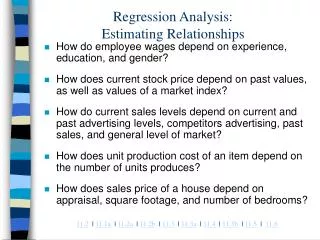
Regression Analysis: Estimating Relationships. How do employee wages depend on experience, education, and gender? How does current stock price depend on past values, as well as values of a market index?

Regression Analysis: Estimating Relationships
E N D
Presentation Transcript
Regression Analysis:Estimating Relationships • How do employee wages depend on experience, education, and gender? • How does current stock price depend on past values, as well as values of a market index? • How do current sales levels depend on current and past advertising levels, competitors advertising, past sales, and general level of market? • How does unit production cost of an item depend on the number of units produces? • How does sales price of a house depend on appraisal, square footage, and number of bedrooms?
Regression Analysis:Estimating Relationships • How does a single variable depend on other relevant variables? • The response (dependent) variable is the variable being explained by the regression. • The explanatory (or independent) variables are used to explain the dependent variable. • Simple regression: Single explanatory variable • Multiple regression: Any number of explanatory variables
Example 11.1Sales Versus Promotions At Pharmex Scatterplots: Graphing Relationships
Objective To use a scatterplot to examine the relationship between promotional expenses and sales at Pharmex.
Background Information • Pharmex is a chain of drugstores that operates around the country. • To see how effective their advertising and other promotional activities are, the company has collected data from 50 randomly selected metropolitan regions. • In each region it has compared its own promotional expenditures and sales to those of the leading competitor in the region over the past year.
Background Information -- continued • There are two variables each of which are indexes, not dollar amounts. • Promote: Pharmex’s promotional expenditures as a percentage of those of the leading competitor • Sales: Pharmex’s sales as a percentage of those of the leading competitor • The company expects that there is a positive relationship between the two variables, so that regions with relatively more expenditures have relatively more sales. However, it is not clear what the nature of this relationship is.
PHARMEX.XLS • The data are listed in this file. Here is a partial listing. • What type of relationship, if any, is apparent in a scatterplot?
Creating the Scatterplot • In preparing to create the scatterplot we must decide which variable should be on the horizontal axis. • In regression analysis, we always put the explanatory variable on the horizontal axis and the response variable on the vertical axis. • In this example the store tends to believe that large promotional expenditures “cause” larger values of sales, so we put Sales on the vertical axis and Promote on the horizontal axis.
Creating the Scatterplot -- continued • We create the following scatterplot using StatPro’s Scatterplot procedure.
Interpretation • The scatterplot indicates that there is a positive relationship between Promote and Sales - the points tend to rise from bottom left to top right - but the relationship is not perfect. • The correlation of 0.673 is shown automatically on the plot. The important things to note about the correlation is that it is positive and its magnitude is moderately large.
Causation • Unless the data is obtained in a carefully controlled experiment - not the case here - we can never make definitive statements about causation in regression analysis. • The reason for this is that we can almost never rule out the possibility that some other variable is causing the variation in both of the observed variables.
Example 11.1Sales Versus Promotions at Pharmex Simple Linear Regression
Objective To use a scatterplot to examine the relationship between promotional expenses and sales at Pharmex.
Background Information • In Example 11.1 we created scatterplots for Pharmex. • We found that there was a positive but not perfect relationship between Promote and Sales. • We now want to find the least squares line for the Pharmex drugstore data, using Sales as the response variable and Promote as the explanatory variable.
PHARMEX.XLS • The data are listed in this file. Here is a partial listing.
Least Squares Estimation • Since there are hints of a linear relationship between the two variables we can draw a line through the points to produce a reasonably good fit. • However, we need to proceed systematically and not just randomly draw lines. We must choose the line that makes the vertical distances from the points to the line as small as possible. • The fitted value is the vertical distance from the horizontal axis to the line and the residual is the vertical distance from the line to the point.
Least Squares Estimation -- continued • The idea is simple. By using a straight line to reflect the relationship between Promote and Sales, we expect a given Sales to be at the height of the line above any particular value of Promote. That is, we expect Sales to equal the fitted value. • But the relationship is not perfect. Not all points lie exactly on the line. The differences are the residuals. They show how much the observed values differ from the fitted values.
Least Squares Estimation -- continued • We can now explain how to choose the “best fitting” line through the points in the scatterplot. We choose the line with the smallest sum of the squared residuals. This line is called the least squares line. • Most statistical packages perform the calculations to find this line so we need not be concerned with the technical details and hand calculating.
Finding the Least Squares Line with StatPro • We use the StatPro/Regression Analysis /Simple menu item. • After specifying that Sales is the response (dependent) variable and that Promote is the explanatory (independent) variable, we see the dialog box for scatterplot options as seen here.
Finding the Least Squares Line with StatPro -- continued • This gives us the option of creating several scatterplots involving the fitted values and residuals. • The regression output includes three parts. The first two are a list of fitted values and residuals, placed in columns next to the data set, and any scatterplots selected from the dialog box. • The third part of the output is the most important. It is shown on the next slide.
The Regression Output • We will eventually learn what all the output in the table means but for now we will concentrate on a small part. • Specifically we find the intercept and slope of the least squares line under the Coefficient label in cells C16 and C17. • They imply that the equation for the least squares line is Predicated Sales = 25.1264 + 0.7623Promote
Least Square Line Equation • We can interpret the regression equation for this example as follows. • The slope 0.7623 indicates that the sales index tends to increase by about 0.76 for each unit increase in the promotional expenses index. • The interpretation of the intercept is less important. It is literally the predicted sales index for a region that does no promotions. • For instances like this when the range of observed explanatory variable values does not include 0, it is best to think of the intercept as an “anchor” for the least squares line.
The Scatterplot • A useful graph in almost any regression analysis is a scatterplot of residuals (on the vertical axis) versus fitted values. • The scatterplot for this data appears on the following slide. • We typically examine the scatterplot for striking patterns. • A “good” fit not only has small residuals, but it has residuals scattered randomly around 0 with no apparent pattern. This is the case here.
The Scatterplot of Residuals versus Fitted Values for Pharmex