Download
1 / 24
240 likes | 366 Views
This presentation by Philip Roe from the University of Michigan discusses a new structure for Lagrangian hydrocodes, emphasizing the limitations of traditional Godunov-type methods used in Eulerian computational fluid dynamics (CFD). The proposed strategy aims to enhance Lagrangian computations by incorporating ideas of symmetry and vorticity while addressing one-dimensional physics limitations. The work introduces a novel method for storing Eulerian and Lagrangian variables, ensuring conservation and stability for complex fluid dynamics problems. The approach is generalized for three-dimensional computations and arbitrary grids, improving information transfer and introducing new stability properties.

E N D
A new structure for LagrangianHydrocodes Philip Roe Department of Aerospace Engineering University of Michigan Ann Arbor Presented at Multimat 2011, Arcachon, France, September 2011
Motivation Godunov-type methods have enjoyed much success in Eulerian CFD and, based on this, are being energetically applied to Lagrangianhydrocodes. But even in the Eulerian context, criticism can be levelled against Godunov methods, especially in their reliance on one-dimensional physics (“Riemann problems”). We will present a new strategy, borrowing from a variety of sources, adapted to Lagrangian computations, and oriented around considerations of symmetry and vorticity.
Objectives, compared to current Godunov schemes Remove One-dimensional physics Retain Conservation (including total energy) Upwinding (proper information transfer) Limiting (to evade Godunov’s theorem) IntroduceVorticity transport (to aid stability) Permitting Generalisation to three dimensions, and arbitrary polygonal/polyhedral grids
One-dimensional physics This is the picture typically associated with finite volume methods, especially Godunov-type methods. It focuses on two cells, and on the flux between them. If uL,uR are both constant and one-dimensional then this flux is obtained by solving the Riemann problem. What is the correct generalisation of this idea? In particular, what is the correct generalisation of the diagram?
1½ - dimensional physics This is the usual version. We focus on a surface because the flux is thought of as passing through a surface. Each surface is most naturally associated with the pair of cells that it separates. This redirects our attention to the Riemann problem and to one-dimensional physics.
An alternative kind of flux Recalling that the flux is actually a vector with x- and y- components (f, g), it might be more appropriate to evaluate that vector at a point, rather than one component of it at a surface. The vector flux must depend on four states, and the corresponding diagram is more two-dimensional in appearance.
An alternative stencil The evaluation of component fluxes naturally leads to a five-point stencil (left), whereas the evaluation of vector fluxes naturally leads to a nine-point stencil (right). For linear advection, the nine-point “rotated Richtmyer” stencil (Richtmyer, 1967) has much superior properties, including a larger stability region and more isotropic properties (which implies less mesh imprinting, Morton and Roe 2001), Moreover, for systems, the five-point stencil cannot enforce two-dimensional properties such as vorticity (MR, Mishra &Tadmor, 2010).
Data structure for Lagrangian hydrodynamics On a logically rectangular grid, it is proposed to store the Eulerian variables (ρ, ρ u, ρ v, E) in cells, and Lagrangian variables (u,v,p) at vertices. The Eulerian variables are integrated conservatively by integrating around the (moving) control volumes. This is straightforward once the Lagrangian variables are known. The Lagrangian variables are updated non-conservatively, by analogy with their linearised form (the acoustic equations). It will be through this aspect that upwinding (correct transmission of information) is imposed.
Double storage • There is no problem attached to storing velocity twice, once at vertices and again in cells (as momentum). • The idea is used in, e.g., van Leer “Toward the ultimate…IV” (JCP, 1977), but also in any high-order scheme that adds degrees of freedom to a cell. • Van LeersSchemes IV and V both use data stored both as cell averages and independently as point fluxes. • They are second order and third order advection schemes with excellent performance. • There is an inconsistent mode that is very rapidly damped. • The illustration shows an extension to the 1D Euler equations of scheme V by Eymann and Roe (AIAA, 2011).
Three-dimensional acoustics and spherical means If a quantity u(x,t) satisfies the three- dimensional wave equation then u(x,t) depends on the initial data only through the data on the surface of the spherer=at, centered on x. Specifically, (Courant and Hilbert II, p 202), where is a mean value on the surface of that sphere. This formula is exact and true for all time. If the data depends only on one coordinate x, it yields the characteristic equations. If the data depends only on two dimensions, the solution depends on both the boundary and the interior of the Mach disk.
Two-dimensional acoustics and circular means In an acoustic problem, the pressure p does satisfy the wave equation, and can be found from the previous formulas. The velocities do not satisfy the wave equation (unless the flow is irrotational) but the solution for them can be obtained by manipulations. To create a second-order numerical scheme it is only required to evaluate the vertex quantities to order Δt. We find, upon specialising to two-dimensional data, It is not so easy to do this in the Eulerian form, which is complicated by the presence of advective terms ɸ
AlgorithmStep 1 • Assume all variables known at the start of the timestep. • Update the Lagrangian variables u, v, p at the vertices by integratinglinearised acoustic solutions over the bilinear distributions within each cell. • The appropriate upwind bias is obtained by evaluating the contribution from each quadrant separately. • Find the trajectory of each vertex and the time-averaged pressure on its path. • This is the stage to introduce limiters, of which, more later.
Algorithm Step 2 The Lagrangian variables u,v, p provide the Eulerian fluxes p, up, vp. Integrating these over the dark shaded areas yields conservation of mass, momentum and total energy, over each cell.
Areas and derivatives The area of a plane quadrilateral is given by Call this function . Given some function defined at the vertices, we can define a discrete gradient This very useful formula is second-order accurate, because it is exact in the special cases . There is a (more complicated) three-dimensional version.
Mesh instability and vorticity • Most Lagrangeanhydrocodes, left to run for long enough, develop severe mesh distortions accompanied by strong spurious vorticity. • Dukowicz and Meltz (JCP, 1992) showed that the distortion was greatly reduced by instituting vorticity control. Their method was expensive and only first order. • For the incompressible case, the circulation round a cell remains constant and the proposed method reproduces this Kelvin theorem (Morton and Roe 2001) • For the compressible case, a correction may be needed.
Evolution of vorticity Vorticityevolution is governed by the transport equation; Integrating this over the cell gives where is the circulation round the cell, and the RHS is the area in the plane . This formula is again second-order by the same argument. If it is obeyed, we have a discrete Kelvin theorem around any contiguous set of cells.
Vorticity control • At the conclusion of a time step, we have new nodal velocities, and new cell circulations from two different calculations. These would agree exactly for a linear problem, but not in the nonlinear case. • We can accept the cell divergence predicted from the vertex calculation, and the cell circulation from the cell update. • These will yield a globalelliptic system for a set of nodal velocities that obey the vorticity evolution equation. • It would be expensive to solve this at every timestep, but a local hyperbolic procedure (Dedner et al, JCP, 2002) seems to be very efficient.
Limiting • All high-order schemes require limiting to evade Godunov’s theorem, and in Godunov-type methods this is usually carried out on solution gradients entering the Riemann solver. • The Flux-corrected transport method (FCT, Boris and Book, JCP, 1972) admits extrema into the solution only if their presence is vouched for by a low-order scheme. • This is a more multidimensional procedure; it can be made very close to gradient limiting in the case of systems having all wavespeeds equal (acoustics, Lagrangean hydro, geometrical shock dynamics) • We have developed a version in which the limiting is not done on velocity gradients, but on velocity divergences.
Comparing gradient limiting and FCT • FCT may be a good candidate for limiting in (single material) Lagrangianhydrocodes, where the wavespeeds at a given interface are almost equal and opposite. • Gradient limiting • Requirescharacteristicdecompositionand/or Riemann solver. • Uses one-dimensional concepts. • Relatively expensive. • Handles systems with different wavespeeds well. • FCT • No decomposition required. • Conceptually independent of dimension • Less expensive. • Deals less well with different wavespeeds..
Comparing gradient limiting and FCT ν = 0.50 ν = 0.25 ν = 0.75 On a simple advection test, there is little to choose between slope limiting with the “double minmod” limiter(○) and FCT (x)
Objectives, compared to current Godunov schemes Remove One-dimensional physics Retain Conservation (including total energy) Upwinding (proper information transfer) Limiting (to evade Godunov’s theorem) IntroduceVorticity transport (to aid stability) Ensuring Generalisation to three dimensions
Remarks • There are many possible ways to put together a CFD code, and by no means have all of them been tried. • The proposal made here differs in many respects from both traditional Lagrangean and regular Godunov methods. • Eulerian variables are stored in cell centers and Lagrangean variables at nodes; these are updated alternately. • Upwinding is introduced by integrals that are exact in the acoustic case, and are distinct from one-dimensional characteristic or compatibility relationships. • Independent evolution of vorticity is easily performed and may help with stability. • Flux-corrected transport may be a preferable way to apply limiting.
Acknowledgements • Don Burton (LANL) for financial support. • Andy Barlow (AWE) and Nikos Nikiforakis (Cambridge) for hospitality in the UK. • PrasannaVaradarajan (UoM) for FCT comparisons.
Evolution of area The evolution of area (and hence τ) is given by 2