Download
1 / 43
440 likes | 672 Views
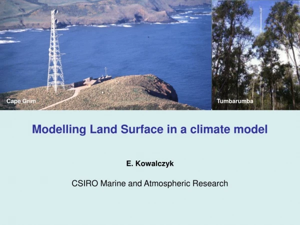
Modelling Land Surface in a climate model. Cape Grim. Tumbarumba. E. Kowalczyk CSIRO Marine and Atmospheric Research. Outline. Role of the land surface schemes (LSS) in climate models Surface energy and water balance in climate model

E N D
Modelling Land Surface in a climate model Cape Grim Tumbarumba E. Kowalczyk CSIRO Marine and Atmospheric Research
Outline • Role of the land surface schemes (LSS) in climate models • Surface energy and water balance in climate model • Representation of vegetation processes in CABLE • Description of land hydrology and soil temperature • - soil moisture & temperature • - snow accumulation, melting and properties • Examples of use of CABLE coupled to a climate model
Time scale of biosphere-atmosphere interactions Physical-chemical forcing T,u,Pr,q, Rs,Rl, CO2 Canopy conductance photosynthesis, leaf respiration Carbon transfer, Soil temp. & moisture availibity Allocation Biogeo- chemical forcing Solution of SEB; canopy and ground temperatures and fluxes Autotrophic and Heterotrophic respiration Atmosphere Vegetation dynamics & disturbance Turnover Land-use and land-cover change Surface water balance Vegetation change Phenology Update LAI, Photosyn-thesis capacity Soil heat and moisture Nutrient cycle Radiation water, heat, & CO2 fluxes Fast biophysical processes Intermediate timescale biogeochemical processes Slow biogeographical processes days years minutes
Role of the Land Surface Scheme (LSS) in GCM LSS calculates exchanges of moisture, energy, momentum and trace gasses at the land-atmosphere interface. Land surface important characteristics for calculation of SEB: albedo, leaf area index, canopy height, surface moisture. Key task is to calculate Surface Energy Balance: L λE S H Tf Tg Snet + Lnet – G = H + λE
Atmosphere-Land Coupling Transpiration Precip. Runoff Evap. Precip Evap iver Changes of land features Infiltration orography, vegetation, albedo, etc Drainage Surface Water Balance in Climate Model Prec –Evap–Runoff=ΔSnow + ΔSoilMoist Land surface important characteristics: soil hydraulic properties & depth vegetation properties; rooting depth leaf area index, max carboxylation rate
The general structure of CABLE SEB & fluxes; for soil-vegetation system: Ef , Hf , Eg , Hg; evapotranspiration Canopy radiation; sunlit & shaded visible & near infra-red, albedo Carbon fluxes;GPP, NPP, NEP stomata transp. & photosynthesis Interface to GCM or offline soil temp. soil moisture soil respiration snow carbon pools; allocation & flow Email:bernard.pak@csiro.au Visit the CABLE secured website with your supplied password athttps://teams.csiro.au/sites/cable/default.aspx Kowalczyk et al., CMAR Research Paper 013, 2006. http://www.cmar.csiro.au/e-print/open/kowalczykea_2006a.pdf
The main features of CABLE • a coupled model of stomatal conductance, photosynthesis and the partitioning of absorbed net radiation into latent and sensible heat fluxes • the model differentiates between sunlit and shaded leaves i.e. two-big-leaf sub-models for calculation of photosynthesis, conductance and leaf temperature • the radiation submodel calculates the absorption of beam and diffuse radiation in visible and near infrared wavebands, and thermal radiation • the vegetation is placed above the ground allowing for full aerodynamic and radiative interaction between vegetation and the ground • the plant turbulence model by Raupach et al. (1997) • a multilayer soil model is used; Richards equations are solved for soil moisture and heat conduction equation for soil temperature • the snow model computes temperature, density and thickness of three snowpack layers. • biogeochemical model CASA CNP for carbon, nitrogen and phosphorus including symbiotic nitrogen fixation ( Wang, Houlton and Field,2007).
Outline • Role of the land surface schemes (LSS) in climate models • Surface energy and water balance in climate model • Representation of vegetation processes in CABLE • Description of land hydrology and soil temperature • - soil moisture & temperature • - snow accumulation, melting and properties • Examples of use of CABLE coupled to a climate model Representation of vegetation processes in CABLE
Canopyrepresentation CABLE
Coupled model of stomatal conductance and photosynthesis The two-leaf model ( sunlit & shaded ) of Wang & Leuning [1998] is used to calculate 6 variables: • Tf - leaf temperature • Ds - vapour pressure deficit • Cs - CO2 concentration at the leaf surface • Ci - intercellular CO2 concentration of the leaf • Gs - stomatal conducatnce • An - net photosynthesis The set of six equations is used to solve simultaneously for photosynthesis, transpiration, leaf temperature and sensible heat fluxes for a each leaf
Vegetation parameters required for CABLE • VEGETATION TYPE • 1 broad-leaf evergreeen trees • 2 broad-leaf deciduous trees • 3 broad-leaf and needle-leaf trees • 4 needle-leaf evergreen trees • 5 needle-leaf deciduous trees • 6 broad-leaf trees with ground cover /short-vegetation/C4 grass (savanna) • 7 perennial grasslands • 8 broad-leaf shrubs with grassland • 9 broad-leaf shrubs with bare soil • 10 tundra • 11 bare soil and desert • agricultural/c3 grassland • 13 ice Geographically explicit data LAI – leaf area index fractional cover C3/C4 - fraction themodel calculates: z0 – roughness length α – canopy albedo A grouping of species that show close similarities in their response to environmental control have common properties such as: - vegetation height - root distribution - max carboxylation rate - leaf dimension and angle, sheltering factor, - leaf interception capacity
Outline • Role of the land surface schemes (LSS) in climate models • Surface energy and water balance in climate model • Representation of vegetation processes in CABLE • Description of land hydrology and soil temperature • - soil moisture & temperature • - snow accumulation, melting and properties • Examples of use of CABLE coupled to a climate model
Multilayer soil model Net Solar + Net Long wave sensible evap ground heat Z1=0.02m Z1 Z2 Z3 ZN-1 ZN-1 ZN ZN Thickness of soil layers (m) 0.022 0.058 0.154 0.409 1.085 2.872
Soil moisture model precipitation + snow melt plant ET soil evap Surface runoff calculated as saturation excess ( + effects of topography if coupled to a climate model) surf runoff Z1 Z2 Z3 ZN-1 Drainagecalculated as excess of soil field capacity or gravitational drainage ZN drainage Soil moisture is calculated from the solution of Richard’s equation. The assumed form of relationship between the hydraulic conductivity, matric potential and the soil moisture is that of Clapp and Hornberger (1978).
Soil Moisture: some terms and concepts Soil moisture : quantity of water in soil, θ = Vwater / Vsoil Є( 0 , 0.5 ) Saturation: water fills in all available pore space Field Capacity: water that remains in soil beyond the effects of gravity. Permanent Wilting: amount of water after the permanent wilting point is reached • Available Water: amount of water • in the soil between the field capacity • and the permanent wilting percentage
Soil parameters required for CABLE Soil Properties: - water balance: saturation wilting point field capacity hydraulic cond. at saturation matric potential at saturation - heat storage: albedo, specific heat, thermal conductivity density - soil depth Soil types: Coarse sand/Loamy sand Medium clay loam/silty clay loam/silt loam Fine clay Coarse-medium sandy loam/loam Coarse-fine sandy clay Medium-fine silty clay Coarse-medium-fine sandy clay loam Organic peat Permanent ice Post, W., and L. Zobler, 2000 Global Soil Types
Variation of hydraulic conductivity with water potential K dry wet
The soil parameters used in the CSIRO climate models. Soil types: • (1) Coarse sand/Loamy sand (5) Coarse-fine sandy clay • (2) Medium clay loam/silty clay loam/silt loam (6) Medium-fine silty clay • (3) Fine clay (7) Coarse-medium-fine sandy clay loam • (4) Coarse-medium sandy loam/loam (8) Organic peat (9) Permanent ice SOIL Type 1 Type 2 Type 3 Type 4 Type 5 Type 6 Type 7 Type 8 • density 1600 1600 1600 1600 1600 1600 1600 1300 soil density kg/m3 • sfc 0.143 0.301 0.367 0.218 0.31 0.37 0.255 0.45 field capacity (m3/m3) • swilt 0.072 0.216 0.286 0.135 0.219 0.283 0.175 0.395 wilting point (m3/m3) • ssat 0.398 0.479 0.482 0.443 0.426 0.482 0.420 0.451 saturation (m3/m3) • hyds*10-6 166.0 4.0 1.0 21.0 2.0 1.0 6.0 800.0 hydraulic cond. at saturation (m/s) • sucs -0.106 -0.591 -0.405 -0.348 -0.153 -0.49 -0.299 -0.356 matric potential at saturation • bch 4.2 7.1 11.4 5.15 10.4 10.4 7.12 5.83b parameter in Clapp-Hornberger relations • clay 0.09 0.30 0.67 0.20 0.42 0.48 0.27 0.17 fraction of clay • sand 0.83 0.37 0.16 0.60 0.52 0.27 0.58 0.13 fraction of sand • silt 0.08 0.33 0.17 0.20 0.06 0.25 0.15 0.70 fraction of silt • css 850 850 850 850 850 850 850 1920 soil specific heat (kJ/kg/K) • dry soil thermal conductivity is calculated as: sand*0.3 + clay*0.25 + silt*0.265 [W/m/K] • Thickness of soil layers (m) 0.022 0.058 0.154 0.409 1.085 2.872
Outline • Role of the land surface schemes (LSS) in climate models • Surface energy and water balance in climate model • Representation of vegetation processes in CABLE • Description of land hydrology and soil temperature • - soil moisture & temperature • - snow accumulation, melting and properties • Examples of use of CABLE coupled to a climate model
Modelling of snow evolution • Snow accumulation • Snow albedo • Snow metamorphism and thermal properties • Snow cover interaction with vegetation • Snow melting Snow - properties - high albedo - good thermal insulator - density increases with time
Modelling of snow evolution • Snow state variables: • temperature • density • age • mass • Snow diagnostic variables: • - snow albedo • depth • effective conductivity Snow - properties - high albedo - good thermal insulator - density increases with time
Overlaying the Snow Albedo Statistics onto the Snow-Free Spatially Complete Albedo Snow-Free Spatially Complete ProductJanuary 2002, 0.86µm Using NISE Snow Extent and Type to Overlay the Snow Albedo Statistics Crystal Schaaf, Boston University)
www.nasa.gov/.../content/95040main_snowcover.jpg The Moderate Resolution Imaging Spectroradiometer (MODIS), flying aboard NASA’s Terra and Aqua satellites, measures snow cover over the entire globe every day, cloud cover permitting. The image shows snow cover (white pixels) across North America from February 2-9, 2002.
SNOWMIP I Col de Porte CSIRO observations
Outline • Role of the land surface schemes (LSS) in climate models • Surface energy and water balance in climate model • Representation of vegetation processes in CABLE • Description of land hydrology and soil temperature • - soil moisture & temperature • - snow accumulation, melting and properties • Examples of use of CABLE coupled to a climate model • for C4MIP phase one study.
Time scale of biosphere-atmosphere interactions Physical-chemical forcing T,u,Pr,q, Rs,Rl, CO2 Canopy conductance photosynthesis, leaf respiration Carbon transfer, Soil temp. & moisture availibity Allocation Biogeo- chemical forcing Solution of SEB; canopy and ground temperatures and fluxes Autotrophic and Heterotrophic respiration Atmosphere Vegetation dynamics & disturbance Turnover Land-use and land-cover change Surface water balance Vegetation change Phenology Update LAI, Photosyn-thesis capacity Soil heat and moisture Nutrient cycle Radiation water, heat, & CO2 fluxes Fast biophysical processes Intermediate timescale biogeochemical processes Slow biogeographical processes days years minutes
Major regulatory mechanisms that lead to either positive or negative feedbacksof C cycle to climate warming Photosynthesis Respiration acclimation acclimation Nutrient availability diminishing Decomposition Length of growing seasons Drought Increased evapotranspiration Warming- or nutrient prone species Stress-tolerant species Negative feedback Neutral Positive feedback Luo Annu. Rev. Ecol. Evol. 2007
CSIRO Carbon-climate simulation • C4MIP phase I simulation: • Coupled CABLE (CSIRO Atmosphere Biosphere Land Exchange LSS) with CCAM (Cubic Conformal Atmospheric Model). • Used prescribed SST, carbon fluxes from ocean, fossil fuel and land use change from 1900 to 2000. • Two atmospheric CO2 concentrations used: 1) prescribed historical CO2 globally uniform, 2) a result of atmospheric transport of all carbon fluxes including biospheric fluxes. • Two simulations: RUN1: biosphere sees prescribed historical CO2 from 1900 to 2000 RUN2: biosphere sees prescribed historical CO2 from 1900 to 1970, then CO2 is kept constant at 1970 level from 1971 to 2000. Law, Kowalczyk & Wang, Tellus, 58B, 427-437, 2006.
Fossil Fuel CO2 emissions fluxes Carbon cycle in C-CAM coupled carbon-climate model C-CAM CO2 atmospheric transport CABLE interface to C-CAM Ocean Carbon fluxes CABLE photosynthesis CO2 uptake CO2 release Phenology heterotrophic respiration Stem Land-use and land-cover change fluxes Soil Carbon Roots hydrology
Conformal-cubic C48 grid used for C4MIP simulations Resolution is about 220 km
Model forcing and modelled climate Sea Surface Temperature: HadISST1.1 dataset, 1x1o, monthly Land air temperature 1900 2000 CO2 concentration Law Dome (pre 1958), then South Pole and Mauna Loa, smoothed 1900 2000 1900 2000
Carbon fluxes through 20th century GPP – photosynthesis increases as atmospheric CO2 increases NPP (photosynthesis minus plant respiration) and soil respiration increase with increasing CO2 NEE (net exchange with atmosphere) starts ~neutral (tuned) and becomes sink 1900 2000
Barrow Ulaan Uul WLEF Mauna Loa Cape Rama South Pole Map of output locations Tapajos Red: atmospheric sampling sites, blue: flux tower sites Atmospheric data ‘see’ CO2 sources/sinks from a larger region than flux towers
Seasonal cycle: amplitude and phase Model Observations Peak to peak amplitude – too low in northern mid-latitudes Month of minimum, out by 4-5 months in southern hemisphere Data: GLOBALVIEW-CO2 (2003)
Barrow Ulaan Uul Mauna Loa Cape Rama Seasonal cycle: NH sites Blue: obs Green: CABLE Red: CASA Data: GLOBALVIEW-CO2 (2003)
Seasonal cycle: southern hemisphere South Pole Contribution of source from each semi-hemisphere Blue: obs, green: model, red: CASA Data: GLOBALVIEW-CO2 (2003)
CO2 at Mauna Loa CO2 concentration (ppm) Model: red, Observed: blue Annual growth of CO2 (ppm/yr) Data: Keeling et al (2005) 1960 2000
CO2 Growth Rate Components at South Pole Station (ppm/yr) Fossil fuel Total Land use Biosphere Ocean
Future plans Conclusions - Model simulated GPP,NPP,RP, Rs increased steadily over 20th century with NEP changing from being slightly positive (source) to being slightly negative (sink) - Tropical rainforest and savanna were main contributors to global NEP variability - CO2 fertilization effect was strongest for tropical forest, savanna and C3 grass/agriculture - Simulated seasonal CO2 cycles were mostly good for Northern hemisphere stations and poor for Southern hemisphere - implement new biogeochemical model - improve vegetation phenology - participate in the 2nd C4MIP experiment
Thank you Eva.kowalczyk@csiro.au
Potentially important feedbacks in coupled climate-carbon cycle system. Response of the terrestrial biosphere to: (-) (+) Albedo (α) Increase in α • increasing CO2 • climate change • climate variability AbsorbedSw decrease Rn increase Rn decrease Increase in α H & EL Cloudiness & Precip. decrease Reduction in Soil moisture Sw increase Example of a simple albedo feedbacks