Download
1 / 40
400 likes | 419 Views
Explore the fundamental hypothesis of equilibrium statistical mechanics and how it relates to the derivation of equilibrium conditions and constraints in statistical thermodynamics. Learn about reversible and irreversible processes and the concept of accessible states. Understand the distribution of energy between systems in equilibrium.

E N D
Statistical Thermodynamics • A slight rewording of the Fundamental Hypothesis of (Equilibrium) Statistical Mechanics: “In a closed system, every (micro-) state is equally likely to be observed”. • A consequence of this is that ALL of Equilibrium Statistical Mechanics & Thermodynamics can be derived!
Equilibrium Conditions & ConstraintsReversible & Irreversible Processes
Consider an isolated macroscopic system A in internal equilibrium with specified energy E. The number of accessible states for Ais Ωi(E). • Suppose that A contains at least one Internal Constraint. ConstraintSystem property that limits the number of accessible states Ωi(E).
Example: Consider a gas in a container which is divided by a partition into 2 equal volumes V. The gas is in equilibrium & is confined by the partition to the left side. See figure: Gas V Vacuum V
Gas V Vacuum V • Remove the Partition:The new • situation is clearlyNOT an equilibrium • one. All accessible states in the right side • are NOT filled. Wait some time. As a result • of collisions between the molecules, • Eventually they distribute themselves uniformly over the entire volume2V.
Gas 2V V • When thepartition is removed,& after we wait until a new equilibrium is reached, the • Molecules eventually will be distributed • uniformly over the entire volume2V. • The new equilibrium is as illustrated in the figure. • Compare initial # of accessible states Ωi(E) the molecules had before removing the partition to final # of accessible states Ωf(E) after removing it. • Clearly, Ωf(E) > Ωi(E).
In this simple example, after the gas comes to a new equilibrium, Ωf(E)> Ωi(E) • More generally, consider an isolated system A, in internal equilibrium at energy E, subject to one or more constraints. The number of accessible states is Ωi(E). • Remove one or more constraints. Except in very special cases, the new situation is NOT an equilibrium one. Wait some time until a new equilibrium is reached as a result of interactions between particles in A.
General Discussion • An isolated system A, in internal equilibrium at energy E, with one or more constraints. Remove one or more constraints. Wait some time until a new equilibrium is reached as a result of interactions between particles in A. • Compare the initial number of accessible states Ωi(E) before removing constraints to the final number of accessible states Ωf(E)after removal. • Generally, it will be true that Ωf(E)> Ωi(E). • In some very special cases, it will be true that Ωf(E)= Ωi(E).
After system A comes to a new equilibrium, it will be true in general that Ωf(E)Ωi(E) • If the equals sign holds, Ωf(E)= Ωi(E)& the removal of the constraint is called a Reversible Process. • If the greater than signholds, Ωf(E)> Ωi(E) & the removal of the constraint is called an Irreversible Process. • A Reversible Process is an idealization! All Real InteractionProcesses are Irreversible!
The figures below illustrate the problem of gas • molecules in a container. But, • The following discussion applies to • essentially any thermodynamic system. • For six molecules in a container, the figures show • three possible spatial configurations of the • molecules. The total number of possible • configurations is huge, of course!!
This microstate is possible,but there aren’t many microstates that give these extreme results. So it is highly improbable! Each individual microstate is equally probable. Consider the FundamentalHypothesis If the number of particles is large (>10)the probability functionsfor this type of configuration are sharply peaked. So this type of configuration is highly probable!
Does the Fundamental Hypothesis lead to something that isConsistent with Classical Thermodynamics? • Assume systems A1 & A2 are weakly • coupled so they can exchange energy. • They correspond to Reif’s systemsA & A'. E2 = E - E1 E1 Calculation of E1 The most probable energy of system A1 E = E1 + E2 • The probability finding of A1with a particular energy E1 • is proportional to the product of the number of accessible • states of A1 times the number of accessible states of A2 • Consistent with Energy Conservation: E = E1 + E2
E2 = E - E1 E = E1 + E2 E1 • Stated another way: • Each configuration is equally probable, • but, the number of states having a particular • energyE1is huge & unknown.We find E1 by • finding the energy where the left side of • the above equation has a maximum.
Some Math Details Start with (1): Take the natural log of both sides: Find E1 where this is max by setting the derivative = 0 (2): Combine (1) & (2):
Combine (1) & (2): Energy is Conserved! dE1 = -dE2 This is the Thermal Equilibrium Condition!! Definition of the parameterβ
So, at Equilibrium, it must be true that: The Thermal Equilibrium Condition!! Definition of β • A Fundamental Statistical Definition! • The physical interpretation of βis that it is a measure of • A System’s Temperature!
Also, DEFINE the EntropyS of a system as: (kB= 1.380662 10-23 J/K = Boltzmann’s constant) In thermodynamics, we DEFINEthe Kelvin Temperature Scalesuch that: But we just defined: So, [1/(kBT)]
This gives a “Statistical” Definition of Temperature: Entropy & Temperatureare both related to the number of accessible states Ω(E). The Fundamental Postulateleads to: 1. An Equilibrium Condition. Two systems are in thermal equilibrium when their temperatures are equal. (Obvious, but we proved it!) 2. A Maximum Entropyfor the coupled systems when they are at equilibrium. As we’ll see, this is related to the The 2nd Law of Thermodynamics. We’ll see all of this in more detail soon. 3. The 3rd Law of Thermodynamics also.
Consider 2 macroscopic systems A, A', interacting & in equilibrium. The combined system A0 = A +A', is isolated. AssumeThermal Interactions Only • Recallthat in a pure • Thermal Interaction, • no mechanical work is • done. So the energy • exchange between A • & A' is a pure A' A Heat Exchange!!
After much tedious derivation, the probability of • finding the combined system A0 = A +A' in a state • for which the system A has an energy E looks like: P(E) ΔE (10-12)Ē ΔE Ē/(f)½ E Ē For f = 1024, (f)½ = 1012, so ΔE Ē/(f)½ (10-12)Ē
Consider 2 macroscopic systems A, A', interacting & in equilibrium. The combined system A0 = A +A', is isolated.Assume • Mechanical Interactions Only • Recallthat in a pure • Mechanical Interaction, • mechanical work is done. So, • the energy exchange between A' A • A, A' occurs becauseThey Do Workon each other! • Recall also that doing mechanical work means that at least • one external parameter (x) of Achanges. Further, this • change in x can be characterized by a generalized force • X -(E/x)
After much tedious derivation, the probability of finding • the combined system A0 = A +A'in a state for which • the system A has a generalized force X looks like: P(X) ΔX <X>/(f)½ ΔX (10-12)<X> X <X> For f = 1024, (f)½ = 1012, so ΔX <X>/(f)½ (10-12)<X>
Example:If the external parameter for a gas is the • volume, x = V, then we’ve already seen that the resulting • generalized force is the gas pressure p, X = p. P(p) Δp (10-12)<p> Δp <p>/(f)½ p <p> For f = 1024, (f)½ = 1012, so Δp <p>/(f)½ (10-12)<p>
Consider 2 macroscopic systems A, A', interacting & in equilibrium. The combined system A0 = A +A', is isolated. Assume that Both Thermal & Mechanical Interactions Occur at the Same Time A A'
The probability of finding the combined system • A0 = A +A' being in a state for which the system • A has energy E is as before. So, P(E) ΔE (10-12)Ē ΔE Ē/(f)½ E Ē For f = 1024, (f)½ = 1012, so ΔE Ē/(f)½ (10-12)Ē
The probability of finding the combined system • A0 = A +A' in a state for which the system A has • a mean generalized force X is as before, so P(X) ΔX <X>/(f)½ ΔX (10-12)<X> X <X> For f = 1024, (f)½ = 1012, so ΔX <X>/(f)½ (10-12)<X>
The Approach to Thermal Equilibrium:Entropy & the 2nd Law ofThermodynamics
As we’ve seen, Entropyis DEFINED as Boltzmann’s constant times the natural log of the number of accessible states S kBlnΩ(E)
Entropyis DEFINED as S kBlnΩ(E) • As already discussed, for two interacting systems, A & A', the number of accessible states can be written: Ω0(E,E') = Ω(E)Ω'(E') • So the entropy of the combined system can be written: S0kBln[Ω0(E,E')] = kBln[Ω(E)Ω'(E')] = kBln[Ω(E)] + kBln[Ω'(E')] or S0 = S(E) + S'(E')
The 2nd Law of Thermodynamics • Consider 2 macroscopic systems A, A', each initially isolated & not interacting with each other. • Define:Ωi(E) ≡Initial number of accessible states at energy E for A. Ω'i(E') Initial number of accessible states at energy E'for A'. • Now, bring A &A' into contact, let them interact & wait long enough that they come to equilibrium. The combined system A0 = A +A', is isolated.
The combined system A0 = A +A', is isolated. • After they come to equilibrium: • Define: Ωf(E) Final number of accessible states at energy E for A. Ω'f(E') Final number of accessible states at energy E'for A'. • As we’ve also seen, it will be true in general for A &A' that Ωf(E)Ωi(E)&Ω'f(E')Ω'i(E')
After systems A &A' come to equilibrium, Ωf(E)Ωi(E)&Ω'f(E')Ω'i(E') • If the equals signs hold, Ωf(E)= Ωi(E) &Ω'f(E')= Ω'i(E') & the interaction of A &A' is called a Reversible Process.
After systems A &A' come to equilibrium, Ωf(E)Ωi(E)& Ω'f(E')Ω'i(E') • If the greater than signs hold, Ωf(E)> Ωi(E) &Ω'f(E')> Ω'i(E'), the interaction of A &A' is called an Irreversible Process. A Reversible Process is an idealization! All Real InteractionProcesses are Irreversible!
In terms of Entropies, S = kBln(Ω), this means that after systemsA &A'come to equilibrium: Sf(E)Si(E)&S'f(E')S'i(E')(1) • If the equals signs hold, Sf(E)=Si(E)& S'f(E')=S'i(E') & the interaction of A &A' is called a Reversible Process.
In terms of Entropies, S = kBln(Ω), this means that after systemsA &A'come to equilibrium: Sf(E)Si(E)&S'f(E')S'i(E') (1) • If the greater than signs hold, Sf(E)>Si(E)&S'f(E')>S'i(E') the interaction of A &A' is called an Irreversible Process.
The Total Entropy of A &A'before they are in contact is: Si = Si(E) +S'i(E') (2) • The Total Entropy of A &A'after they are in contact is: Sf = Sf(E) + S'f(E') (3) • Taking (1), (2), & (3) together clearly means that, after a new equilibrium is reached, it will always be true that: SfSiorΔS 0
Summary • If any 2 macroscopic systems A, A', each initially isolated, in internal equilibrium & not interacting with each other are brought into contact & allowed to interact, AND • If enough time has passed that they’ve come to a new equilibrium, it is always true that: SfSiorΔS 0
If enough time has passed that they’ve come to a new equilibrium, it is always true that: SfSiorΔS 0 • That is, The Total Entropy S of the 2 systems will always either increase or remain the same. This is called The 2nd Law of Thermodynamics