Download
1 / 129
1.29k likes | 1.35k Views
Chap.17 Biogeography. 鄭先祐 (Ayo) 教授 國立台南大學 環境與生態學院 生態科學與技術學系 環境生態 + 生態旅遊 ( 碩士班 ). 17 Biogeography. Case Study: The Largest Ecological Experiment on Earth Biogeography and Spatial Scale Global Biogeography Regional Biogeography Case Study Revisited

E N D
Chap.17 Biogeography 鄭先祐 (Ayo) 教授 國立台南大學 環境與生態學院 生態科學與技術學系 環境生態 + 生態旅遊 (碩士班)
17 Biogeography Case Study: The Largest Ecological Experiment on Earth Biogeography and Spatial Scale Global Biogeography Regional Biogeography Case Study Revisited Connections in Nature: Human Benefits of Tropical Rainforest Diversity
Case Study: The Largest Ecological Experiment on Earth One hectare of rainforest in the Amazon contains more plant species than all of Europe! The Amazon Basin is the largest watershed in the world. The number of fish species in the Amazon River exceeds the total number found in the entire Atlantic Ocean.
Figure 17.1 Diversity Abounds in the Amazon Freshwater fish caught in the Amazon river on display in a market in Manaus, Brazil.
Case Study: The Largest Ecological Experiment on Earth When these ecosystems are disturbed, there is devastating species loss. Deforestation began with road building in the 1960s. In 50 years’ time, 15% of the rainforest has been converted to pastureland, towns, roads, and mines.
Case Study: The Largest Ecological Experiment on Earth While 15% seems modest, the sheer number of species impacted is staggering. The pattern of deforestation has also resulted in extreme habitat fragmentation, making it more difficult to maintain species diversity.
Figure 3.6 Tropical Deforestation June 22, 1992 June 19, 1975 August 1, 1986 February 7, 2001
Case Study: The Largest Ecological Experiment on Earth In 1979, habitat fragmentation spurred Thomas Lovejoy to initiate the longest running ecological experiment ever conducted: The Dynamics of Forest Fragments Project (BDFFP). He was guided by The Theory of Island Biogeography, an explanation for the observation that more species are found on large islands than on small islands.
Case Study: The Largest Ecological Experiment on Earth Four different sizes of forest plots were set up: 1, 10, 100, or 1,000 hectares. Control plots were surrounded by forest. Fragments were surrounded by logged land. The BDFFP started with the question, “What is the minimum area of rainforest needed to maintain species diversity?”
Figure 17.2 Studying Habitat Fragmentation in Tropical Rainforests Plots of four sizes-- 1, 10, 100, 1,000 hectares-- were designated before logging took place. Control plots remained surrounded by forested land. (B) Aerial photo of a 1 ha and 10 ha fragment isolated in 1983. Experimental fragments were surrounded by deforested land.
Introduction Physical factors and species interactions are important regulators of species distributions on local scales. But global and regional scale processes are also important in determining the distributions and diversity of species on Earth.
Biogeography and Spatial Scale Concept 17.1: Patterns of species diversity and distribution vary at global, regional, and local spatial scales. Biogeography is the study of patterns of species composition and diversity across geographic locations.
Biogeography and Spatial Scale A tour of the forest biomes of the world reveals the huge variation in species richness and composition. The Amazon rainforest is the most species-rich forest in the world, with approximately 1,300 tree species. In contrast, the boreal forests of Canada have only 2 tree species that cover vast areas.
Figure 17.3 Forests around the World (C) Lowland temperate forest in the Pacific Northwest. (A) A tropical rainforest in Brazil (D) Boreal spruce forest in northern Canada. (B) Oak woodland in southern California
Biogeography and Spatial Scale New Zealand has been separated from continental land masses for about 80 million years. Since that time evolution has resulted in unique forests. About 80% of the species are endemic, meaning that they occur nowhere else on Earth.
Biogeography and Spatial Scale Even within New Zealand there is a range of tree species composition and richness. North Island is warmer, with many flowering tree species, and some emergent conifers. The kauri(貝殼杉) (Agathis australis) is among the largest tree species on Earth.
Biogeography and Spatial Scale The kauri trees(貝殼杉)have been extensively logged, and exist in only two small reserves. Old-growth stands of kauris take 1,000–2,000 years to generate, so these forests are irreplaceable to modern society.
Biogeography and Spatial Scale The forest tour reveals several patterns: Species richness and composition vary with latitude. In general, the lower tropical latitudes have many more, and different, species than the higher temperate and polar latitudes.
Biogeography and Spatial Scale Species richness and composition also vary from continent to continent, even where longitude or latitude is roughly similar. The same community type or biome can vary in species richness and composition depending on its location on Earth.
Biogeography and Spatial Scale Ecologists have worked to understand the processes that control these broad patterns. A number of hypotheses have been proposed, which are highly dependent on spatial scale.
Biogeography and Spatial Scale Spatial scales are interconnected in a hierarchical way, with the patterns of species diversity and composition at one spatial scale setting the conditions for patterns at smaller spatial scales.
Figure 17.5 Interconnected Spatial Scales of Species Diversity Global patterns of species diversity and composition are driven by variation in speciation, extinction, and migration rates across latitudes and longitudes. Within regions, patterns of species diversity and composition are driven by migration and extinction rates across the landscape. The local and regional scales are connected by turnover, the difference in species number and composition as one moves across the landscape from one community type to another. Local patterns of species diversity and composition are driven by physical conditions and species interactions.
Biogeography and Spatial Scale Global scale —the entire world. Species have been isolated from one another, on different continents or in different oceans, by long distances and over long periods. Rates of speciation, extinction, and migration help determine differences in species diversity and composition.
Biogeography and Spatial Scale Regional scale —climate is roughly uniform and the species are bound by dispersal to that region. Regional species pool—all the species contained within a region (gamma diversity).
Biogeography and Spatial Scale Landscape—topographic and environmental features of a region. Species composition and diversity vary within a region depending on how the landscape shapes rates of migration and extinction to and from critical local habitats.
Biogeography and Spatial Scale Local scale —equivalent to a community. Species physiology and interactions with other species weigh heavily in the resulting species diversity (alpha diversity).
Biogeography and Spatial Scale Beta diversity —change in species number and composition, or turnover of species, as one moves from one community type to another. Beta diversity represents the connection between local and regionalscales of species diversity.
Biogeography and Spatial Scale Actual area values of the different spatial scales depends on the species and communities of interest. Example: Terrestrial plants might have a local scale of 102–104 m2, but for phytoplankton, the local scale might be more like 102 cm2.
Biogeography and Spatial Scale Patterns of species diversity, and the processes that control them, are interconnected across spatial scales. The regional species pool provides the raw material for local assemblages and sets the theoretical upper limit on species diversity for communities.
Biogeography and Spatial Scale Three types of relationships between local and regional diversity: 1. When regional and local species diversity are equal (slope = 1), all species in a region will be found in all communities. This is not really likely, as regions will always have landscape and habitat features that exclude some species from some communities.
Figure 17.6 What Determines Local Species Diversity? When local and regional species diversity values are equal (slope=1), then all the species within a region will be found in all communities of that region. When local diversity values are lower than regional diversity values, but still increase with them proportionally (slope<1), regional processes dominate over local processes. If local diversity stays the same as regional diversity increases (the curve levels off), local processes limit local diversity.
Biogeography and Spatial Scale 2. If local species richness is simply proportional to regional species richness, community species richness is largely determined by the regional species pool. 3. If local species richness levels off despite a large regional species pool, then local processes can be assumed to limit local species diversity.
Biogeography and Spatial Scale Witman et al. (2004) looked at invertebrate communities on subtidal rock walls at 49 local sites in 12 regions around the world. A plot of all local sites showed that local species richness was always proportionally lower than regional species richness and that it never leveled off.
Figure 17.7 Marine Invertebrate Communities May Be Limited by Regional Processes (Part 1) Among shallow sub tidal marine invertebrate communities, regional species richness explains approximately 75% of the local species richness. (A) The 12 regions of the world where the 49 sampling sites were located.
Figure 17.7 Marine Invertebrate Communities May Be Limited by Regional Processes (Part 2) The slop of the line is less than 1, suggesting that regional species pools largely determine local species richness.
Biogeography and Spatial Scale Regional species richness explained 75% of the variation in local species richness. But this does not mean that local processes are unimportant. There is still considerable unexplained variation that could be attributable to the effects of local processes.
Biogeography and Spatial Scale The effects of species interactions, in particular, are likely to be highly sensitive to the local spatial scale chosen. Inappropriate (usually too large) spatial scales are unlikely to detect local effects.
Global Biogeography Biogeography was born with scientific exploration in the 19th century. Alfred Russel Wallace (1823–1913) rightly earned his place as the father of biogeography. Concept 17.2: Global patterns of species diversity and composition are controlled by geographic area and isolation, evolutionary history, and global climate.
Figure 17.8 Alfred Russel Wallace and His Collections (A) a photograph of Wallace taken in Singapore in 1862, during his expedition to the Malay Archipelago. (B) Some of Wallace's rare beetle collections from the Malay Archipelago found in an attic by his grandson in 2005.
Global Biogeography Wallace is best known, along with Charles Darwin, as the codiscoverer of the principles of natural selection. But his main contribution was the study of species distributions across large spatial scales.
Global Biogeography While working in the Malay Archipelago, Wallace noticed that the mammals of the Philippines were more similar to those in Africa (5,500 km away) than they were to those in New Guinea (750 km away).
Figure 8.10 Continental Drift Affects the Distribution of Organisms
Global Biogeography Wallace published The Geographical Distribution of Animalsin 1876. Wallace overlaid species distributions and geographic regions and revealed two important global patterns: Earth’s land mass can be divided into six biogeographic regions. The gradient of species diversity with latitude.
Global Biogeography The six biogeographic regions correspond roughly to Earth’s six major tectonic plates. The plates are sections of Earth’s crust that move or drift (continental drift) through the action of currents generated deep within the molten rock mantle.
Figure 17.10 Mechanisms of Continental Drift 地殼 岩漿 At subduction zones, one plate is forced under another. 地幔 At mid-ocean ridge, molten rock flows from Earth's mantle to form new crust, pushing plates apart.
Global Biogeography At mid-ocean ridges, the molten rock flows out of the seams between plates and cools, creating new crust and forcing the plates to move apart. At subduction zones, one plate is forced downward under another plate. These areas are associated with strong earthquakes, volcanic activity, and mountain range formation.
Global Biogeography In other areas where two plates meet, the plates slide sideways past each other, forming a fault (斷層). The positions of the plates, and the continents that sit on them, have changed dramatically over geologic time. For biogeography, we will consider continental drift since the end of the Permian period, 250 million years ago.