Computing Engine Choices

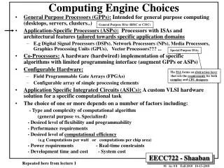
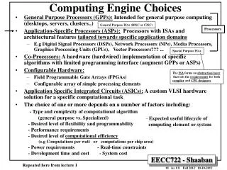
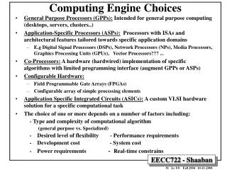
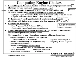
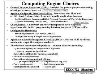
1. Computing Engine Choices General Purpose ISAs (RISC or CISC) • General Purpose Processors (GPPs): Intended for general purpose computing (desktops, servers, clusters..) • Application-Specific Processors (ASPs): Processors with ISAs and architectural features tailored towards specific application domains • E.g Digital Signal Processors (DSPs), Network Processors (NPs), Media Processors, Graphics Processing Units (GPUs), Vector Processors??? ... • Co-Processors: A hardware (hardwired) implementation of specific algorithms with limited programming interface (augment GPPs or ASPs) • Configurable Hardware: • Field Programmable Gate Arrays (FPGAs) • Configurable array of simple processing elements • Application Specific Integrated Circuits (ASICs): A custom VLSI hardware solution for a specific computational task • The choice of one or more depends on a number of factors including: - Type and complexity of computational algorithm (general purpose vs. Specialized) - Desired level of flexibility and programmability - Performance requirements - Desired level of computational efficiency (e.g Computations per watt or computations per chip area) - Power requirements - Real-time constraints - Development time and cost - System cost Special Purpose ISAs

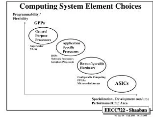
2. Computing Engine Choices • e.g Digital Signal Processors (DSPs), • Network Processors (NPs), • Media Processors, • Graphics Processing Units (GPUs) • Physics Processor …. General Purpose Processors (GPPs): Flexibility Processor = Programmable computing element that runs programs written using a pre-defined set of instructions Application-Specific Processors (ASPs) Programmability / Configurable Hardware Selection Factors: • Type and complexity of computational algorithm • (general purpose vs. Specialized) • - Desired level of flexibility and programmability • - Performance requirements • - Desired level of computational efficiency • Power requirements - Real-time constraints • - Development time and cost - System cost Co-Processors Application Specific Integrated Circuits (ASICs) Specialization , Development cost/time Performance/Chip Area/Watt (Computational Efficiency)

3. Why Application-Specific Processors (ASPs)? Computing Element Choices Observation • Generality and efficiency are in some sense inversely related to one another: • The more general-purpose a computing element is and thus the greater the number of tasks it can perform, the less efficient (e.g. Computations per chip area /watt) it will be in performing any of those specific tasks. • Design decisions are therefore almost always compromises; designers identify key features or requirements of applications that must be met and and make compromises on other less important features. • To counter the problem of computationally intense and specialized problems for which general purpose machines cannot achieve the necessary performance/other requirements: • Special-purpose processors (or Application-Specific Processors, ASPs) , attached processors, and coprocessors have been designed/built for many years, for specific application domains, such as image or digital signal processing (for which many of the computational tasks are specialized and can be very well defined). Generality = Flexibility = Programmability ? Efficiency = Computations per watt or chip area

4. Digital Signal Processor (DSP) Architecture • Classification of Main Processor Types/Applications • Requirements of Embedded Processors • DSP vs. General Purpose CPUs • DSP Cores vs. Chips • Classification of DSP Applications • DSP Algorithm Format • DSP Benchmarks • Basic Architectural Features of DSPs • DSP Software Development Considerations • Classification of Current DSP Architectures and example DSPs: • Conventional DSPs: TI TMSC54xx • Enhanced Conventional DSPs: TI TMSC55xx • Multiple-Issue DSPs: • VLIW DSPs: TI TMS320C62xx, TMS320C64xx • Superscalar DSPs: LSI Logic ZSP400/500 DSP core

5. Main Processor Types/Applications • General Purpose Computing & General Purpose Processors (GPPs) – • High performance: In general, faster is always better. • RISC or CISC: Intel P4, IBM Power4, SPARC, PowerPC, MIPS ... • Used for general purpose software • End-user programmable • Real-time performance may not be fully predictable (due to dynamic arch. features) • Heavy weight, multi-tasking OS - Windows, UNIX • Normally, low cost and power not a requirement (changing) • Servers, Workstations, Desktops (PC’s), Notebooks, Clusters … • Embedded Processing: Embedded processors and processor cores • Cost, power code-size and real-time requirements and constraints • Once real-time constraints are met, a faster processor may not be better • e.g: Intel XScale, ARM, 486SX, Hitachi SH7000, NEC V800... • Often require Digital signal processing (DSP) support or other application-specific support (e.g network, media processing) • Single or few specialized programs – known at system design time • Not end-user programmable • Real-time performance must be fully predictable (avoid dynamic arch. features) • Lightweight, often realtime OS or no OS • Examples: Cellular phones, consumer electronics .. … • Microcontrollers • Extremely code size/cost/power sensitive • Single program • Small word size - 8 bit common • Usually no OS • Highest volume processors by far • Examples: Control systems, Automobiles, industrial control, thermostats, ... Increasing Cost/Complexity Increasing volume Examples of Application-Specific Processors (ASPs)

6. The Processor Design Space Application specific architectures for performance Embedded processors Microprocessors GPPs Real-time constraints Specialized applications Low power/cost constraints Performance is everything & Software rules Performance Microcontrollers Cost is everything Chip Area, Power complexity Processor Cost

7. Requirements of Embedded Processors • Usually must meet strict real-time constraints: • Real-time performance must be fully predictable: • Avoid dynamic processor architectural features that make real-time performance harder to predict ( e.g cache, dynamic scheduling, hardware speculation …) • Once real-time constraints are met, a faster processor is not desirable (overkill) due to increased cost/power requirements. • Optimized for a single (or few) program (s) - code often in on-chip ROM or on/off chip EPROM/flash memory. • Minimum code size (one of the motivations initially for Java) • Performance obtained by optimizing datapath • Low cost • Lowest possible area • High computational efficiency: Computation per unit area • VLSI implementation technology usually behind the leading edge • High level of integration of peripherals (System-on-Chip -SoC- approach reduces system cost/power) • Fast time to market • Compatible architectures (e.g. ARM family) allows reusable code • Customizable cores (System-on-Chip, SoC). • Low power if application requires portability

8. Embedded Processors Area of processor cores = Cost (and Power requirements) Nintendo processor Cellular phones

9. Embedded Processors Another figure of merit: Computation per unit area (Computational Efficiency) Nintendo processor Cellular phones

10. Embedded Processors Smaller is better Code size • If a majority of the chip is the program stored in ROM, then minimizing code size is a critical issue • Common embedded processor ISA features to minimize code size: • Variable length instruction encoding common: • e.g. the Piranha has 3 sized instructions - basic 2 byte, and 2 byte plus 16 or 32 bit immediate • Complex/specialized instructions • Complex addressing modes

11. Embedded Systems vs. General Purpose Computing Embedded Systems General Purpose Computing Systems (and embedded processors) (and processors GPPs) Used for general purpose software : Intended to run a fully general set of applications that may not be known at design time Run a single or few specialized applications often known at system design time May require application-specific capability (e.g DSP) No application-specific capability required Not end-user programmable End-user programmable Minimum code size is highly desirable Minimizing code size is not an issue Heavy weight, multi-tasking OS - Windows, UNIX Lightweight, often real-time OS or no OS Low power and cost constraints/requirements Higher power and cost constraints/requirements • Usually must meet strict real-time constraints • (e.g. real-time sampling rate) In general, no real-time constraints • Real-time performance must be fully predictable: • Avoid dynamic processor architectural features that make real-time performance harder to predict • Real-time performance may not be fully predictable (due to dynamic processor architectural features): • Superscalar: dynamic scheduling, hardware speculation, branch prediction, cache. Once real-time constraints are met, a faster processor is not desirable (overkill) due to increased cost/power requirements. Faster (higher-performance) is always better

12. Evolution of GPPs and DSPs • General Purpose Processors (GPPs) trace roots back to Eckert, Mauchly, Von Neumann (ENIAC) • Digital Signal Processors (DSPs) are microprocessors designed for efficient mathematical manipulation of digital signals utilizing digital signal processing algorithms. • DSPs usually process infinite continuous sampled data streams (signals) while meeting real-time and power constraints. • DSPs evolved from Analog Signal Processors (ASPs) that utilize analog hardware to transform physical signals (classical electrical engineering) • ASP to DSP because: • DSP insensitive to environment (e.g., same response in snow or desert if it works at all) • DSP performance identical even with variations in components; 2 analog systems behavior varies even if built with same components with 1% variation • Different history and different applications requirements led to different terms, different metrics, architectures, some new inventions. + EDSAC

13. DSP vs. General Purpose CPUs • DSPs tend to run one (or few) program(s), not many programs. • Hence OSes (if any) are much simpler, there is no virtual memory or protection, ... • DSPs usually run applications with hard real-time constraints: • DSP must meet application signal sampling rate computational requirements: • A faster DSP is overkill (higher DSP cost, power..) • You must account for anything that could happen in a time slot (DSP algorithm inner-loop, data sampling rate) • All possible interrupts or exceptions must be accounted for and their collective time be subtracted from the time interval. • Therefore, exceptions are BAD. • DSPs usually process infinite continuous data streams: • Requires high memory bandwidth (with predictable latency, e.g no data cache) for streaming real-time data samples and predictable processing time on the data samples • The design of DSP ISAs and processor architectures is driven by the requirements of DSP algorithms. • Thus DSPs are application-specific processors

14. DSP vs. GPP i.e Main performance measure of DSPs is MAC speed • The “MIPS/MFLOPS” of DSPs is speed of Multiply-Accumulate (MAC). • MAC is common in DSP algorithms that involve computing a vector dot product, such as digital filters, correlation, and Fourier transforms. • DSP are judged by whether they can keep the multipliers busy 100% of the time and by how many MACs are performed in each cycle. • The "SPEC" of DSPs is 4 algorithms: • Inifinite Impule Response (IIR) filters • Finite Impule Response (FIR) filters • FFT, and • convolvers • In DSPs, target algorithms are important: • Binary compatibility not a major issue • High-level Software is not as important in DSPs as in GPPs. • People still write in assembly language for a product to minimize the die area for ROM in the DSP chip. Why? Note: While this is still mostly true, however, programming for DSPs in high level languages (HLLs) has been gaining more acceptance due to the development of more efficient HLL DSP compilers in recent years.

15. Types of DSP Processors According to type of Arithmetic/operand Size Supported • 32-BIT FLOATING POINT (5% of DSP market): • TI TMS320C3X, TMS320C67xx (VLIW) • AT&T DSP32C • ANALOG DEVICES ADSP21xxx • Hitachi SH-4 • 16-BIT FIXED POINT (95% of DSP market): • TI TMS320C2X, TMS320C62xx (VLIW) • Infineon TC1xxx (TriCore1) (VLIW) • MOTOROLA DSP568xx, MSC810x (VLIW) • ANALOG DEVICES ADSP21xx • Agere Systems DSP16xxx, Starpro2000 • LSI Logic LSI140x (ZPS400) superscalar • Hitachi SH3-DSP • StarCore SC110, SC140 (VLIW)

16. DSP Cores vs. Chips DSP are usually available as synthesizable cores or off-the- shelf packaged chips • Synthesizable Cores: • Map into chosen fabrication process • Speed, power, and size vary • Choice of peripherals, etc. (SoC) • Requires extensive hardware development effort. • Off-the-shelf packaged chips: • Highly optimized for speed, energy efficiency, and/or cost. • Limited performance, integration options. • Tools, 3rd-party support often more mature SOC = System On Chip Resulting in more development time and cost

17. Time Frame Approach Primary Application Enabling Technologies Early 1970’s · · · Discrete logic Non-real time Bipolar SSI, MSI processing · FFT algorithm · Simulation Late 1970’s · · · Building block Military radars Single chip bipolar multiplier · · Digital Comm. Flash A/D m m Early 1980’s · · · Single Chip DSP P Telecom P architectures · Control · NMOS/CMOS Late 1980’s · · · Function/Application Computers Vector processing specific chips · · Communication Parallel processing Early 1990’s · · · Multiprocessing Video/Image Processing Advanced multiprocessing · VLIW, MIMD, etc. Late 1990’s · · · Single-chip Wireless telephony Low power single-chip DSP multiprocessing · Internet related · VLIW/Multiprocessing DSP ARCHITECTUREEnabling Technologies First microprocessor DSP TI TMS 32010 1 2 3 4 Generations of single-chip (microprocessor) DSPs

18. Texas Instruments TMS320 Family Multiple DSP P Generations 1 2 3 4 (VLIW) Generations of single-chip (microprocessor) DSPs

19. Digital audio applications MPEG Audio Portable audio Digital cameras Cellular telephones Wearable medical appliances Storage products: disk drive servo control Military applications: radar sonar DSP Applications • Industrial control • Seismic exploration • Networking: (Telecom infrastructure) • Wireless • Base station • Cable modems • ADSL • VDSL • …... Current DSP Killer Applications: Cell phones and telecom infrastructure

20. DSP Algorithms & Applications

21. Another Look at DSP Applications • High-end: • Military applications (e.g. radar/sonar) • Wireless Base Station - TMS320C6000 • Cable modem • Gateways • Mid-range: • Industrial control • Cellular phone - TMS320C540 • Fax/ voice server • Low end: • Storage products - TMS320C27 (hard drive controllers) • Digital camera - TMS320C5000 • Portable phones • Wireless headsets • Consumer audio • Automobiles, thermostats, ... Increasing Cost Increasing volume

22. DSP range of applications & Possible Target DSPs

23. Cellular Phone System 1 2 3 4 5 6 7 8 9 0 415-555-1212 CONTROLLER RF MODEM PHYSICAL LAYER PROCESSING BASEBAND CONVERTER A/D SPEECH ENCODE SPEECH DECODE DAC Example DSP Application

24. Cellular Phone: HW/SW/IC Partitioning MICROCONTROLLER 1 2 3 4 5 6 7 8 9 0 415-555-1212 CONTROLLER RF MODEM PHYSICAL LAYER PROCESSING BASEBAND CONVERTER ASIC A/D SPEECH ENCODE SPEECH DECODE DAC DSP ANALOG IC Example DSP Application

25. S/P RAM DMA DSP CORE Mapping Onto System-on-Chip (SoC) (Cellular Phone) S/P phone book keypad intfc protocol DMA control RAM µC speech quality enhancment voice recognition ASIC LOGIC RPE-LTP speech decoder de-intl & decoder Viterbi equalizer demodulator and synchronizer Example DSP Application

26. Example Cellular Phone Organization C540 (DSP) ARM7 (µC) Example DSP Application

27. Graphics Out Uplink Radio Video I/O Downlink Radio Voice I/O Pen In µP Video Unit custom Coms Memory DSP Multimedia System-on-Chip (SoC) e.g. Multimedia terminal electronics • Future chips will be a mix of processors, memory and dedicated hardware for specific algorithms and I/O ASIC Co-processor Or ASP (ASIC) Example DSP Application

28. DSP Algorithm Format • DSP culture has a graphical format to represent formulas. • Like a flowchart for formulas, inner loops, not programs. • Some seem natural:  is add, X is multiply • Others are obtuse: z–1 means take variable from earlier iteration (delay). • These graphs are trivial to decode

29. DSP Algorithm Notation • Uses “flowchart” notation instead of equations • Multiply is or X • Add is or + • Delay/Storage is or or Delay z–1 D

30. Typical DSP Algorithm:Finite-Impulse Response (FIR) Filter • Filters reduce signal noise and enhance image or signal quality by removing unwanted frequencies. • Finite Impulse Response (FIR) filters compute: where • x is the input sequence • y is the output sequence • h is the impulse response (filter coefficients) • N is the number of taps (coefficients) in the filter • Output sequence depends only on input sequence and impulse response.

31. Typical DSP Algorithms:Finite-impulse Response (FIR) Filter • N most recent samples in the delay line (Xi) • New sample moves data down delay line • Filter “Tap” is a multiply-add • Each tap (N taps total) nominally requires: • Two data fetches • Multiply • Accumulate • Memory write-back to update delay line • Special addressing modes (e.g modulo) • Goal: At least 1 FIR Tap / DSP instruction cycle (Multiply And Accumulate, MAC) • Requires real-time data sample streaming • Predictable data bandwidth/latency • Special addressing modes • Repetitive computations, multiply and accumulate (MAC) • Requires efficient MAC support

32. X . . . . hN-1 hN-2 h1 h0 Y Delay (accumulator register) FINITE-IMPULSE RESPONSE (FIR) FILTER A Filter Tap One FIR Filter Tap i.e. Vector dot product Performance Goal: at least 1 FIR Tap / DSP instruction cycle DSP must meet application signal sampling rate computational requirements: A faster DSP is overkill (more cost/power than really needed)

33. Sample Computational Rates for FIR Filtering FIR Type 1-D 1-D 2-D 2-D (4.37 GOPs) 2-D (23.3 GOPs) 1-D FIR has nop = 2N and a 2-D FIR has nop = 2N2. OP = Operation • DSP must meet application signal sampling rate computational requirements: • A faster DSP is overkill (higher DSP cost, power..)

34. FIR filter on (simple) General Purpose Processor loop: lw x0, 0(r0) lw y0, 0(r1) mul a, x0,y0add y0,a,b sw y0,(r2) inc r0 inc r1 inc r2 dec ctr tst ctr jnz loop • Problems: • Bus / memory bandwidth bottleneck, • control/loop code overhead • No suitable addressing modes, instructions - • e.g. multiply and accumulate (MAC) instruction • + GPP Real-time performance may (to meet signal sampling rate) not be fully predictable (due to dynamic processor architectural features): • Superscalar: dynamic scheduling, hardware speculation, branch prediction, cache.

35. Typical DSP Algorithms:Infinite-Impulse Response (IIR) Filter • Infinite Impulse Response (IIR) filters compute: • Output sequence depends on input sequence, previous outputs, and impulse response. • Both FIR and IIR filters • Require vector dot product (multiply-accumulate) operations • Use fixed coefficients • Adaptive filters update their coefficients to minimize the distance between the filter output and the desired signal. i.e Filter coefficients: a(k), b(k) MAC

36. Typical DSP Algorithms:Discrete Fourier Transform (DFT) • The Discrete Fourier Transform (DFT) allows for spectral analysis in the frequency domain. • It is computed as for k = 0, 1, … , N-1, where • x is the input sequence in the time domain • y is an output sequence in the frequency domain • The Inverse Discrete Fourier Transform is computed as • The Fast Fourier Transform (FFT) provides an efficient method for computing the DFT.

37. Typical DSP Algorithms:Discrete Cosine Transform (DCT) • The Discrete Cosine Transform (DCT) is frequently used in image & video compression (e.g. JPEG, MPEG-2). • The DCT and Inverse DCT (IDCT) are computed as: where e(k) = 1/sqrt(2) if k = 0; otherwise e(k) = 1. • A N-Point, 1D-DCT requires N2MAC operations.

38. DSP BENCHMARKS • DSPstone: University of Aachen, application benchmarks • ADPCM TRANSCODER - CCITT G.721, REAL_UPDATE, COMPLEX_UPDATES • DOT_PRODUCT, MATRIX_1X3, CONVOLUTION • FIR, FIR2DIM, HR_ONE_BIQUAD • LMS, FFT_INPUT_SCALED • BDTImark2000: Berkeley Design Technology Inc • 12 DSP kernels in hand-optimized assembly language: • FIR, IIR, Vector dot product, Vector add, Vector maximum, FFT …. • Returns single number (higher means faster) per processor • Use only on-chip memory (memory bandwidth is the major bottleneck in performance of embedded applications). • EEMBC (pronounced “embassy”): EDN Embedded Microprocessor Benchmark Consortium • 30 companies formed by Electronic Data News (EDN) • Benchmark evaluates compiled C code on a variety of embedded processors (microcontrollers, DSPs, etc.) • Application domains: automotive-industrial, consumer, office automation, networking and telecommunications BDTI

39. 4th Generation 3rd Generation 2nd Generation > 800x Faster than first generation 1st Generation

40. Basic ISA/Architectural Features of DSPs DSP ISA Feature • Data path configured for DSP algorithms • Fixed-point arithmetic (most DSPs) • Modulo arithmetic (saturation to handle overflow) • MAC- Multiply-accumulate unit(s) • Hardware rounding support • Multiple memory banks and buses - • Harvard Architecture • Multiple data memories • Specialized addressing modes • Bit-reversed addressing • Circular buffers • Specialized instruction set and execution control • Zero-overhead loops • Support for fast MAC • Fast Interrupt Handling • Specialized peripherals for DSP DSP Architectural Features DSP Architectural Feature Usually with no data cache for predictable fast data sample streaming DSP ISA Feature DSP Architectural Feature Dedicated address generation units are usually used DSP ISA Feature To meet real-time signal sampling/processing constraints - (System on Chip - SoC style) DSP Architectural Feature

41. DSP ISA Features DSP Data Path: Arithmetic • DSPs dealing with numbers representing real world signals=> Want “reals”/ fractions • DSPs dealing with numbers for addresses=> Want integers • DSP ISA (and DSP) must Support “fixed point” as well as integers . -1 Š x < 1 S DSP ISA Feature radix point In DSP ISAs: Fixed-point arithmetic must be supported, floating point support is optional and is much less common . –2N–1 Š x < 2N–1 S radix point Usually 16-bit

42. DSP ISA Features DSP Data Path: Precision • Word size affects precision of fixed point numbers • DSPs have 16-bit, 20-bit, or 24-bit data words • Floating Point DSPs cost 2X - 4X vs. fixed point, slower than fixed point • DSP programmers will scale values inside code • SW Libraries • Separate explicit exponent • “Blocked Floating Point” single exponent for a group of fractions • Floating point support simplify development for high-end DSP applications. 16-bit most common In DSP ISAs: Fixed-point arithmetic must be supported, floating point support is optional and is much less common

43. DSP ISA Feature DSP Data Path: Overflow • DSP are descended from analog : • Modulo Arithmetic. • Set to most positive (2N–1–1) or most negative value(–2N–1) : “saturation” • Many DSP algorithms were developed in this model. 2N–1–1 Saturation Why Support? Due to physical nature of signals –2N–1 Saturation

44. DSP Data Path: Specialized Hardware DSP Architectural Features • Specialized hardware functional units performs all key arithmetic operations in 1 cycle, including: • Shifters • Saturation • Guard bits • Rounding modes • Multiplication/addition (MAC) • 50% of instructions can involve multiplier=> single cycle latency multiplier • Need to perform multiply-accumulate (MAC) fast • n-bit multiplier => 2n-bit product

45. Multiplier Multiplier Shift ALU ALU Accumulator Accumulator G DSP Data Path: Accumulator • Don’t want overflow or have to scale accumulator • Option 1: accumalator wider than product: “guard bits” • Motorola DSP: 24b x 24b => 48b product, 56b Accumulator • Option 2: shift right and round product before adder } MAC Unit

46. DSP Data Path: Rounding Modes • Even with guard bits, will need to round when storing accumulator into memory • 3 DSP standard options (supported in hardware) • Truncation: chop results=> biases results up • Round to nearest: < 1/2 round down,  1/2 round up (more positive)=> smaller bias • Convergent: < 1/2 round down, > 1/2 round up (more positive), = 1/2 round to make lsb a zero (+1 if 1, +0 if 0)=> no biasIEEE 754 calls this round to nearest even

47. DSP Processor Specialized hardware performs all key arithmetic operations in 1 cycle. e.g MAC Hardware support for managing numeric fidelity: Shifters Guard bits Saturation Data Path Comparison General-Purpose Processor • Multiplies often take>1 cycle • Shifts often take >1 cycle • Other operations (e.g., saturation, rounding) typically take multiple cycles.

48. TI 320C54x DSP (1995) Functional Block Diagram Multiple memory banks and buses MAC Unit Hardware support for rounding/saturation

49. Instruction Memory Data Memory First Commercial DSP (1982): Texas Instruments TMS32010 • 16-bit fixed-point arithmetic • Introduced at 5Mhz (200ns) instruction cycle. • “Harvard architecture” • separate instruction, data memories • Accumulator • Specialized instruction set • Load and Accumulate • Two-cycle (400 ns) Multiply-Accumulate (MAC) time. Processor Datapath: Mem T-Register Multiplier P-Register ALU Accumulator

50. First Generation DSP P Texas Instruments TMS32010 - 1982 Features • 200 ns instruction cycle (5 MIPS) • 144 words (16 bit) on-chip data RAM • 1.5K words (16 bit) on-chip program ROM - TMS32010 • External program memory expansion to a total of 4K words at full speed • 16-bit instruction/data word • single cycle 32-bit ALU/accumulator • Single cycle 16 x 16-bit multiply in 200 ns • Two cycle MAC (5 MOPS) • Zero to 15-bit barrel shifter • Eight input and eight output channels