Linear Programming Modeling and Optimization Guide
Learn how to model and solve linear programming problems efficiently. Understand the standard form, converting non-standard forms, and working with algorithms such as Simplex. Enhance your skills for real-world applications.

Linear Programming Modeling and Optimization Guide
E N D
Presentation Transcript
LINEAR PROGRAMMING Modeling a problem is boring --- and a distraction from studying the abstract form! However, modeling is very important: --- for your motivation, --- and for your training on how to use the theory on a real application! Read the text book modeling of a LP problem (Ch 19, introductory material) linear programming
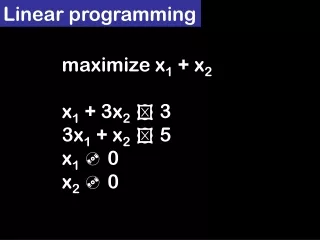
Linear Programming: Standard Form Output: Find values for n variables x1, x2, …, xn: Input: Maximize (j=1n cj xj) (Maximize the objective function) Subject to constraints: j=1n aij xj bi, for i = 1, … m (subject to m linear constraints, and) for all j = 1,…n, xj 0 (all variables are non-negative) The constant coefficients are cj, aij, and bi (input values). Problem size: (n, m). linear programming
Example 1: Maximize (2x1 –3x2 +3x3) Three constraints: x1+x2 –x3 7, -x1 –x2 +x3 -7, x1–2x2 +2x34 Resulting variable values must be positive: x1, x2, x30 Linear Programming: Standard Form linear programming
Non-standard to Standard Form • Note: In the standard form the inequalities must be strict (‘,’ rather than ‘>’), equations are linear (power of x is 0 or 1) • 1) Objective function minimizes as opposed to maximizes • Example 2.1: minimize (-2x1 + 3x2) • Action: Change the signs of coefficients • Example 2.1: maximize (2x1 –3x2) linear programming
Non-standard to Standard Form • 2) Some variables need not be non-negative • Example 2.2: • Constraints: x1 +x2 = 7, x1 –2x2 4, x10, but no constraint on x2. • Action: replace occurrence of any unconstrained variable xj, with a new expression (xj’ – xj’’), and add two new constraints xj’, xj’’ 0. • Example 2.2: • Constraints: x1 +x2’ –x2’’ = 7, x1 –2x2’ +2x2’’ 4, x1, x2’, x2’’ 0. • The number of variables in the problem may at most be doubled, from n to 2n, a polynomial-time increase. linear programming
3) There may be equality constraints Example 2.3: Constraint: x1 +x2 –x3 = 7 Action: replace each equality-linear constraint with two new constraint with , and , and same left and right hand sides. Example 2.3: Two new constraints: x1 +x2 –x3 7, and x1 +x2 –x3 7. Total number of constraints may at most be doubled, from m to 2m, a polynomial-time increase. Non-standard to Standard Form linear programming
4) There may be linear constraints involving ‘’ rather than ‘’ as required by the standard form. Example 2.4: Constraint: x1 +x2 –x3 7 Action: Change the sign of the coefficients (as in the case 1). Example 2.4: New constraint replacing the old one: -x1 –x2 +x3 -7. (Note that now the example 2 is the same as example 1) Note that these form changes do not change the solution of the problem, or They are equivalent forms Equivalent forms of an LP have the same solution as the original one. Non-standard to Standard Form linear programming
Simplex algorithm, Khachien’s algorithm, Karmarkar’s algorithm solves LP. First one is worst-case exp-time algorithm, other two are poly-time algorithms. Simplex: A non-null region in the Cartesian space over the variables, such that any point within the region satisfies the constraints. Algorithms for LP x2 • Five linear constraints together confine a simplex Simplex x1 linear programming
Simplex algorithm iteratively moves from one corner point of the simplex to another trying to increase the value of the optimizing function Solution: where the objective function z has largest value Algorithms for LP Objective Function As a line => Five linear constraints Algorithm wants to take the line further away from the origin Obj. Function value: z x1 linear programming
Solution: where the objective function z has largest value The optimum value of the optimizing function exists at some boundary (a corner point) It may be on infinite number of points over a line (or hyperplane) of the simplex, if the objective function’s line is parallel to a constraint’s line Algorithms for LP Objective Function As a line Algorithm moves from corner to corner of simplex => Five linear constraints Maximum Obj. Func value: z x1 linear programming
Simplex is not a bounded region: Algorithms for LP x2 • Four linear constraints • Simplex is unbounded • No solution, or solution is at infinite point • Objective function can be infinitely increased Simplex x1 linear programming
When the constraints are unsatisfiable the simplex does not exist (or simplex is a nullregion): Algorithms for LP No Simplex x2 • Four linear constraints • Simplex does not exist • No solution, or constraints are conflicting x1 linear programming
Slack Form of a Standard Form: for Simplex Algorithm • Simplex algorithm works with the slack forms (defined below) of an input LP, the latter changes with iterations. • Slack form is equivalent to the input, or, has the same solution. Slack Form of a standard form of LP: • (1) Create a variable z for optimizing function (j=1ncjxj): • z = v + (j=1ncjxj), v is a constant (in the initial slack form v=0) • (2) For each linear constraint (j=1naijxj bi,1im) do introduce an extra variable xj+i and rewrite the constraints: • xj+i = bi - j=1naijxj, 1 i m • (3) Now, only constraints are over the variables, including the new ones (but not on z). • For all variables, xj 0, 1 j n+m linear programming
Example: Slack Form of a Standard Form linear programming
Iterations within Simplex Algorithm • LP in slack form is to find a coordinate in the first quadrant where the value of z is maximum. • Note that the slack forms are non-standard. • Simplex algorithm modifies one slack form to another (i) until z cannot be increased any more, or (ii) terminates when a solution cannot be found. linear programming
Iterations within Simplex Algorithm • Two types of variables: basic variables (B) on left side of the equations, and non-basic variables (N)on the right-hand side . • Example: • Objective functions becomes: z = 0 +3x1 +x2 +2x3 • Linear constraints become equations: x4 = 30 -x1 -x2 -3x3 x5 = 24 -2x1 -2x2 -5x3 x6 = 36 -4x1 -x2 -2x3 • Variable constraints: x1, x2, x3, x4, x5, x6 0 • Two types of variables’ Sets: Non-basic={x1, x2, x3}, Basic={x4, x5, x6} linear programming
Pivoting: trying to increase z value (from 0 now) • z = 0 +3x1 +x2 +2x3 Linear equations: x4 = 30 -x1 -x2 -3x3 x5 = 24 -2x1 -2x2 -5x3 x6 = 36 -4x1 -x2 -2x3 • Constraints: x1, x2, x3, x4, x5, x6 0 Sets: Non-basic={x1, x2, x3}, Basic={x4, x5, x6} • We start with x1=0, x2=0, x3=0 • To increase the value of z: • A non-basic variable whose coefficient is positive in the expression for z can be increased. • In example above, any non-basic variable is a candidate. • We arbitrarily choose x1. • This choice is called the entering variable xein pivot. Our choice xe = x1. linear programming
Pivoting: trying to increase z value (from 0 now) • z = 0 +3x1 +x2 +2x3 Linear equations: x4 = 30 -x1 -x2 -3x3 x5 = 24 -2x1 -2x2 -5x3 x6 = 36 -4x1 -x2 -2x3 • Constraints: x1, x2, x3, x4, x5, x6 0 Sets: Non-basic={x1, x2, x3}, Basic={x4, x5, x6} • Entering variable xein pivot (“entering” in the basic set). • Our choice xe = x1. • If the other non-basic variables hold their value to 0: x1 can be increased up to 30 without violating constraint on x4, x1 can be increased up to 12 without violating constraint on x5, x1 can be increased up to 9 without violating constraint on x6. • So, x6 is the most constraining basic variable. • x6 is chosen as the leaving variable xl by the pivot, xl = x6. linear programming
Iterations within Simplex Algorithm • Only non-basic variables appear in z. • In the initial slack form, original variables are the non-basic variables. • So, the solution we are seeking is the coordinate for those variables where z is max. • Example: • z = 0 +3x1 +x2 +2x3 • Linear equations: x4 = 30 -x1 -x2 -3x3 • x5 = 24 -2x1 -2x2 -5x3 • x6 = 36 -4x1 -x2 -2x3 • Constraints: x1, x2, x3, x4, x5, x6 ≥0 • Sets: N={x1, x2, x3}, B={x4, x5, x6} • Simplex algorithm shuffles variables between the sets N and B, exchanging one variable in N with another in B, in each iteration, with the objective of increasing the value of z. • This operation is the core of the algorithm, and is called the pivot operation. • Moving from corner to corner of the simplex region linear programming
Pivot Algorithm: Core of Simplex z = 0 +3x1 +x2 +2x3 Linear equations: x4 = 30 -x1 -x2 -3x3 x5 = 24 -2x1 -2x2 -5x3 x6 = 36 -4x1 -x2 -2x3 Constraints: x1, x2, x3, x4, x5, x6 0 Sets: N={x1, x2, x3}, B={x4, x5, x6} A basic solution is the coordinates where you put all non-basic variables as 0, and the basic variables are determined for those. So, for this example - the basic solution at the initial stage is: (x1 = 0, x2 = 0, x3 = 0, x4 = 30, x5 = 24, x6 = 36). This basic solution is called feasible since all variables are non-negative. At this point z=0. The pivot operation’s objective is to increase z. linear programming
Example of Pivoting • z = 0 +3x1 +x2 +2x3 Linear equations: x4 = 30 -x1 -x2 -3x3 x5 = 24 -2x1 -2x2 -5x3 x6 = 36 -4x1 -x2 -2x3 • Constraints: x1, x2, x3, x4, x5, x6 0 Sets: N={x1, x2, x3}, B={x4, x5, x6} • A non-basic variable whose coefficient is positive in the expression for z can be increased to increase the value of z. • In example above, any non-basic variable is a candidate. • We arbitrarily choose x1. • This choice is called the entering variable xein pivot. Our choice xe = x1. • If the other non-basic variables hold their value to 0,as in the basic solution: x1 can be increased up to 30 without violating constraint on x4, x1 can be increased up to 12 without violating constraint on x5, x1 can be increased up to 9 without violating constraint on x6. • So, x6 is the most constraining basic variable. • x6 is chosen as the leaving variable xl by the pivot, xl = x6. linear programming
Pivot exchanges xe (x1) and xl (x6) between the sets N and B. Write an equation for x1 in terms of x2, x3, and x6. x6 = 36 -4x1 -x2 -2x3 => x1 =9 + x2/4 + x3/2 -x6/4 Replace x1 with this new expression wherever else x1 appears. The new slack form for the example after this pivot operation is: z = 27 +(1/4)x2 +(1/2)x3 -(3/4)x6 [now, max for z, i.e., v=27] x1 = 9 –(1/4)x2 –(1/2)x3 –(1/4)x6 x4 = 21 –(3/4)x2 –(5/2)x3 +(1/4)x6 x5 = 6 –(3/2)x2 -4x3 +(1/2)x6 x1, x2, x3, x4, x5, x6 0 N={x2, x3, x6}, B={x1, x4, x5} Basic solution after this pivot operation is: (x1, x2, x3, x4, x5, x6) = (9, 0, 0, 21, 6, 0). z at this point is 27, increased from 0 that was in the previous slack form. For the next pivot candidates for the entering variable are x2 and x3 with positive coefficientsin z Pivoting steps linear programming
Pivoting steps • z = 27 +(1/4)x2 +(1/2)x3 -(3/4)x6 [now, max for z, i.e., v=27] • For the next pivot candidates for the entering variable are x2 and x3 with positive coefficients. • If xe=x3 is chosen, then the leaving variable is xl=x5. • Pivot will be applied similarly as before exchanging x3 and x5 from N and B. linear programming
Stopping of Pivoting Iterations in Simplex • Simplex algorithm stops pivoting when none of the coefficients for non-basic variables in z is non-negative. • This indicates that the final solution has been found. • Optimum value for the initial objective function of the standard form LP is the last value of v in z of this terminating slack form. • The basic solution at this point provides the coordinates for initial non-basic variables (x1, x2, and x3, in our example) where this optimum value v for the objective function can be found. • For the example above: • final basic solution is (8, 4, 0, 18, 0, 0) where v=28. • So, the optimum value for the objective function is 28 at (x1=8, x2=4, x3=0). linear programming
Complexity of Simplex • Questions to ask: • How many polygon corners in (n+m)-dimensional space? • Plynomial, but… • Is there any pattern in pivot operation moving from one corner to another? • No pattern, without heuristics • Etc…. • Worst case: O(n22n), for n variables – exponential (but the problem was not NP-hard, eventually proved to be P-class) • Average case: O(n3) • Actual run time depends on Pivoting policy: which +ve coefficient to pick for “entering variable” selection, tie-braking • There exists an efficient policy thattakes 3m pivoting operations http://www.iip.ist.i.kyoto-u.ac.jp/member/cuturi/Teaching/ORF522/lec8v2.pdf linear programming
Complexity of Simplex • “Guessing” LP to be P-class problem, researchers attempted decades trying to prove (or find pivoting policies) to make simplex algo polynomial • However, every policy seems to have a counter example-type with exponential number of steps • Hence, in real-life problem instances Simplex algorithm is very efficient, compared to typical interior point algorithm O(n3.5) • Some exceptional problems “could” be solved by the latter that was not practicable with simplex • Lower bound of LP is O(n) http://www.iip.ist.i.kyoto-u.ac.jp/member/cuturi/Teaching/ORF522/lec8v2.pdf linear programming
Initialization of Simplex • Initialization simplex creates and returns the first slack form. • (1) Init-simplex does a complex operation of checking if the constraints are satisfiable or not (in case the corresponding initial basic solution is not feasible, because one of the variables has negative value). • (2) Init-simplex returns a modified equivalent slack form for which the basic solution is feasible. • (3) Otherwise, init-simplex terminates simplex because no solution may exist for the input. linear programming
Auxiliary problem LAUX • x0 is forcing v=0 within z in the original problem • Objective function from the original problem is eliminated • Purpose: looking for first feasible solution/point • Hoping the point exists, else… • Constraints are conflicting: output “infeasible” • Init-simplex uses Simplex algorithm • Remove x0 terms from final slack form, add expression for z linear programming
Ignore this slide: on anti-cycling Simplex …. https://www.math.washington.edu/~burke/crs/407/lectures/L8-initialization.pdf linear programming
Simplex Algorithm Steps • (1) Init-simplex checks for feasibility, - if so, returns first slack form • (2) Simplex iteratively chooses xe and xl and keeps calling pivot algorithm. • (3) If at a stage none of the basic variables is constrained (can increase unbounded as the xe increases), then no xl exist at that stage. • This indicates the input is unbounded, or the objective function can become infinity. The region simplex is not bounded. Simplex terminates. • (4) Simplex terminates when none of the coefficients of basic variables in z for that iteration is non-negative and returns the optimum value (v) and the solution co-ordinates. linear programming
Simplex algorithm has exponential time-complexity in the worst case, but runs very efficiently on most of the input. (n+m)Choosem pivoting iterations Otherwise, Simplex is in cycle Simplex algorithm may go into infinite loop over pivoting (v remains same from slack form to slack form), but number of pivoting iterations has the above guaranteed upper bound. Proof of the simplex algorithm’s correctness uses the dual LP form. Facts: Simplex Algorithm linear programming
Dual LP linear programming
Primal vs. Dual LP: Proof Sketch of optimal result from Simplex • Dual LP is not an equivalent problem of the primal. • Dual LP is a minimization problem. • Lemma of weak duality: (j=1n cj xj) (i=1m bi yi), for all feasible solutions of both the primal and dual LP’s. • Corollary: When (j=1n cj xj) = (i=1m bi yi) (say,) = v, then v is the optimal value for each of the primal and dual LP. • When the simplex algorithm terminates with none of the coefficients of the basic variables in z as non-negative, then this corollary is satisfied, thus, proving that the algorithm returns optimal value for the objective function of the primal input LP. linear programming
Relation between Primal and Dual Problems Interior-point method (IPM) algorithms work simultaneously on Primal and Dual problem, thus having polynomial-time convergence: Khachiyan’s ellipsoid method O(n6) Karmarkar’s interior-point: O(n3.5) combines both ellipsoid and simplex advantages An IPM Prima-Dual (path finding) Algorithm: https://www.me.utexas.edu/~jensen/ORMM/supplements/methods/lpmethod/S4_interior.pdf IPM opened up a (not-so-new) directions in optimization problems linear programming

