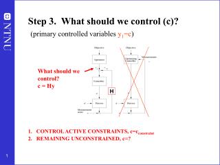
Step 3. What should we control (c)? (primary controlled variables y 1 =c )

1. What should we control? c = Hy Step 3. What should we control (c)?(primary controlled variables y1=c) • CONTROL ACTIVE CONSTRAINTS, c=cconstraint • REMAINING UNCONSTRAINED, c=? H

2. H

3. 2. UNCONSTRAINED VARIABLES:- WHAT MORE SHOULD WE CONTROL?- WHAT ARE GOOD “SELF-OPTIMIZING” VARIABLES? • Intuition: “Dominant variables” (Shinnar) • Is there any systematic procedure? A. Sensitive variables: “Max. gain rule” (Gain= Minimum singular value) B. “Brute force” loss evaluation C. Optimal linear combination of measurements, c = Hy

4. Unconstrained optimum Optimal operation Cost J Jopt copt Controlled variable c

5. Unconstrained optimum Optimal operation Cost J d Jopt n copt Controlled variable c Two problems: • 1. Optimum moves because of disturbances d: copt(d) • 2. Implementation error, c = copt + n

6. Good Good BAD Unconstrained optimum Candidate controlled variables c for self-optimizing control Intuitive • The optimal value of c should be insensitive to disturbances (avoid problem 1) 2. Optimum should be flat (avoid problem 2 – implementation error). Equivalently: Value of c should be sensitive to degrees of freedom u. • “Want large gain”, |G| • Or more generally: Maximize minimum singular value,

7. Guidelines for CV Selection • Rule 1: The optimal value for CV c should be insensitive to disturbances d (minimizes effect of setpoint error) • Rule 2: c should be easy to measure and control (small implementation error n) • Rule 3: c should be sensitive to changes in u (large gain |G| from u to c)orequivalently the optimum Jopt should be flat with respect to c (minimizes effect of implementation error n) • Rule 4: For case of multiple CVs, the selected CVs should not be correlated. Reference: S. Skogestad, “Plantwide control: The search for the self-optimizing control structure”, Journal of Process Control, 10, 487-507 (2000).

8. Unconstrained optimum Quantitative steady-state: Maximum gain rule G c u Maximum gain rule (Skogestad and Postlethwaite, 1996): Look for variables that maximize the scaled gain (Gs) (minimum singular value of the appropriately scaled steady-state gain matrix Gsfrom u to c)

9. cost J u uopt Proof of maximum gain rule Local Loss • Consider Taylor series expansion of J(u,d) around the moving optimal point (uopt(d), d), when u differs from uopt(d) • Ignoring higher order terms • Let G be the (unscaled) steady-state gain matrix

10. Proof of maximum gain rule • Conclusion: To minimize the loss we want to maximize the “scaled gain”:

11. Why is Large Gain Good? J, c Loss Jopt G copt Variation of u c-copt uopt u With large gain G: Even large implementation error n in c translates into small deviation of u from uopt(d) - leading to lower loss

12. Select CVs that maximize (Gs) Maximum Gain Rule in words In words, select controlled variables c for which the gain G (= “controllable range”) is large compared to its span (= sum of optimal variation and control error)

13. Procedure Maximum Gain rule Analysis • Process with • nd (important) disturbances • nu unconstrained degrees of freedom • Several candidate sets of controlled variables c • From a (nonlinear) model, compute the optimal inputs (uopt) and outputs (copt) for different disturbances Need nd + 1 optimizations For each candidate output c, compute the optimal variation copt = (ciopt,max - ciopt,min)/2 • Perturb in each input to find for each candidate c the gain, c = G u • Need nu simulations • Determine the implementation error ni for each candidate output ci • Use engineering knowledge • Scaling matrix for outputs: S1=diag{1/|copti|+|ni|} • If possible: Scale the inputs such that a unit deviation from the optimal value has same effect on J (this makes Juu=I); otherwise compute Juu by perturbing u around the optimal • Select those outputs as controlled variables, which has a large

14. EXAMPLE: Recycle plant(Luyben, Yu, etc.) Recycle of unreacted A (+ some B) 5 Feed of A 4 1 Given feedrate F0 and column pressure: 2 3 Dynamic DOFs: Nm = 5 Column levels: N0y = 2 Steady-state DOFs: N0 = 5 - 2 = 3 Product (98.5% B)

15. Recycle plant: Optimal operation mT 1 remaining unconstrained degree of freedom

16. Control of recycle plant:Conventional structure (“Two-point”: xD) LC LC xD XC XC xB LC Control active constraints (Mr=max and xB=0.015) + xD

17. Luyben rule Luyben rule (to avoid snowballing): “Fix a stream in the recycle loop” (F or D)

18. Luyben rule: D constant LC LC XC LC Luyben rule (to avoid snowballing): “Fix a stream in the recycle loop” (F or D)

19. A. Maximum gain rule: Steady-state gain Conventional: Looks good Luyben rule: Not promising economically

20. How did we find the gains in the Table? • Find nominal optimum • Find (unscaled) gain G0 from input to candidate outputs:  c = G0 u. • In this case only a single unconstrained input (DOF). Choose at u=L • Obtain gain G0 numerically by making a small perturbation in u=L while adjusting the other inputs such that the active constraints are constant (bottom composition fixed in this case) • Find the span for each candidate variable • For each disturbance di make a typical change and reoptimize to obtain the optimal ranges copt(di) • For each candidate output obtain (estimate) the control error (noise) n • The expected variation for c is then: span(c) = i |copt(di)| + |n| • Obtain the scaled gain, G = |G0| / span(c) • Note: The absolute value (the vector 1-norm) is used here to "sum up" and get the overall span. Alternatively, the 2-norm could be used, which could be viewed as putting less emphasis on the worst case. As an example, assume that the only contribution to the span is the implementation/measurement error, and that the variable we are controlling (c) is the average of 5 measurements of the same y, i.e. c=sum yi/5, and that each yi has a measurement error of 1, i.e. nyi=1. Then with the absolute value (1-norm), the contribution to the span from the implementation (meas.) error is span=sum abs(nyi)/5 = 5*1/5=1, whereas with the two-norn, span = sqrt(5*(1/5^2) = 0.447. The latter is more reasonable since we expect that the overall measurement error is reduced when taking the average of many measurements. In any case, the choice of norm is an engineering decision so there is not really one that is "right" and one that is "wrong". We often use the 2-norm for mathematical convenience, but there are also physical justifications (as just given!). IMPORTANT!

21. B. “Brute force” loss evaluation: Disturbance in F0 Luyben rule: Conventional Loss with nominally optimal setpoints for Mr, xB and c

22. B. “Brute force” loss evaluation: Implementation error Luyben rule: Loss with nominally optimal setpoints for Mr, xB and c

23. Conclusion: Control of recycle plant Active constraint Mr = Mrmax Self-optimizing L/F constant: Easier than “two-point” control Assumption: Minimize energy (V) Active constraint xB = xBmin

24. Recycle systems: Do not recommend Luyben’s rule of fixing a flow in each recycle loop (even to avoid “snowballing”)

25. Summary: Procedure selection controlled variables • Define economics and operational constraints • Identify degrees of freedom and important disturbances • Optimize for various disturbances • Identify active constraints regions (off-line calculations) For each active constraint region do step 5-6: 5. Identify “self-optimizing” controlled variables for remaining degrees of freedom 6. Identify switching policies between regions

26. Conditions for switching between regions of active constraints • Within each region of active constraints it is optimal to • Control active constraints at ca = c,a, constraint • Control self-optimizing variables at cso = c,so, optimal • Define in each region i: • Keep track of ci (active constraints and “self-optimizing” variables) in all regions i • Switch to region i when element in ci changes sign • Research issue: can we get lost?

27. Example switching policies – 10 km • ”Startup”: Given speed or follow ”hare” • When heart beat > max or pain > max: Switch to slower speed • When close to finish: Switch to max. power Another example: Regions for LNG plant (see Chapter 7 in thesis by J.B.Jensen, 2008)

28. Comments • Evaluation of candidates can be time-consuming using general non-linear formulation • Pre-screening using local methods. • Final verification for few promising alternatives by evaluating actual loss • Maximum gain rule is extremely simple and insightful, but “may” lead to non-optimal set of CVs • The maximum gain rule assumes that the worst-case setpoint errors Δci,opt(d) for each CV can appear together. In general, Δci,opt(d) are correlated. • Exact local methods (worst-case or average-case) are more accurate • Lower loss: measurement combinations as CVs (next)

29. H

30. Unconstrained degrees of freedom: Ideal “Self-optimizing” variables • Operational objective: Minimize cost function J(u,d) • The ideal “self-optimizing” variable is the gradient (first-order optimality condition (ref: Bonvin and coworkers)): • Optimal setpoint = 0 • BUT: Gradient can not be measured in practice • Possible approach: Estimate gradient Ju based on measurements y • Approach here: Look directly for c as a function of measurements y (c=Hy) without going via gradient

31. Optimal measurement combination • Candidate measurements (y): Include also inputs u H So far: H is a ”selection matrix” [0 0 1 0 0] Now: H is a full ”combination matrix”

32. Optimal measurement combinations Nullspace method (no noise) H = ? Basis: Want optimal value of c to be independent of disturbances • Find optimal solution as a function of d: uopt(d), yopt(d) • Linearize this relationship: yopt= F d • Want: • To achieve this for all values of  d: • To find a F that satisfies HF=0 we must require • Optimal when we disregard implementation error (n) Amazingly simple! Sigurd is told how easy it is to find H V. Alstad and S. Skogestad, ``Null Space Method for Selecting Optimal Measurement Combinations as Controlled Variables'', Ind.Eng.Chem.Res, 46 (3), 846-853 (2007).

33. Unconstrained degrees of freedom: Nullspace method continued • To handle implementation error: Use “sensitive” measurements, with information about all independent variables (u and d)

34. Unconstrained degrees of freedom: Optimal measurement combination 2. “Exact local method” (Combined disturbances and implementation errors) Theorem 1. Worst-case loss for given H(Halvorsen et al, 2003): Applies to any H (selection/combination) Theorem 2 (Alstad et al. ,2009): Optimization problem to find optimal combination is convex. • V. Alstad, S. Skogestad and E.S. Hori, ``Optimal measurement combinations as controlled variables'', Journal of Process Control, 19, 138-148 (2009).

35. Toy Example Reference: I. J. Halvorsen, S. Skogestad, J. Morud and V. Alstad, “Optimal selection of controlled variables”, Industrial & Engineering Chemistry Research, 42 (14), 3273-3284 (2003).

36. Toy Example: Measurement combinations

37. Toy Example

38. Example: CO2 refrigeration cycle pH • J = Ws (work supplied) • DOF = u (valve opening, z) • Main disturbances: • d1 = TH • d2 = TCs (setpoint) • d3 = UAloss • What should we control?

39. CO2 refrigeration cycle Step 1. One (remaining) degree of freedom (u=z) Step 2. Objective function. J = Ws (compressor work) Step 3. Optimize operation for disturbances (d1=TC, d2=TH, d3=UA) • Optimum always unconstrained Step 4. Implementation of optimal operation • No good single measurements (all give large losses): • ph, Th, z, … • Nullspace method: Need to combine nu+nd=1+3=4 measurements to have zero disturbance loss • Simpler: Try combining two measurements. Exact local method: • c = h1 ph + h2 Th = ph + k Th; k = -8.53 bar/K • Nonlinear evaluation of loss: OK!

40. CO2 cycle: Maximum gain rule

41. Refrigeration cycle: Proposed control structure Control c= “temperature-corrected high pressure”

42. The rest in not part of the syllabus for the course

43. 2. General (with noise). “Exact local method” Loss L = J(u,d) – Jopt(d). Keep c = Hy constant , where y = Gyu + Gydd + ny Theorem 1. Worst-case loss for given H(Halvorsen et al, 2003): Applies to any H (selection/combination) Optimization problem for optimal combination: • I.J. Halvorsen, S. Skogestad, J.C. Morud and V. Alstad, ``Optimal selection of controlled variables'', Ind. Eng. Chem. Res., 42 (14), 3273-3284 (2003).

44. Theorem 2. Explicit formula for optimal H. (Alstad et al, 2008): • F – optimal sensitivity matrix = dyopt/dd Theorem 3. (Kariwala et al, 2008). V. Alstad, S. Skogestad and E.S. Hori, ``Optimal measurement combinations as controlled variables'', Journal of Process Control, 18, in press (2008). V. Kariwala, Y. Cao, S. jarardhanan, “Local self-optimizing control with average loss minimization”, Ind.Eng.Chem.Res., in press (2008)

45. Toy Example again Reference: I. J. Halvorsen, S. Skogestad, J. Morud and V. Alstad, “Optimal selection of controlled variables”, Industrial & Engineering Chemistry Research, 42 (14), 3273-3284 (2003).

46. B2. Exact local method (with noise)

47. B2. Exact local method, 2 measurements Combined loss for disturbances and measurement errors

48. B2. Exact local method, all 4 measurements

49. Current research (Henrik Manum):Self-optimizing control and Explicit MPC • Our results on optimal measurement combination (keep c = Hy constant) • Nullspace method for n=0 (Alstad and Skogestad, 2007) • Explicit expression (“exact local method”) for n≠0 (Alstad et al., 2008) • Observation 1: Both result are exact for quadratic optimization problems • Observation 2: MPC can be written as a quadratic optimization problem and optimal solution is to keep c = u – Kx constant. • Must be some link!

50. Quadratic optimization problems • Noise-free case (n=0) • Reformulation of nullspace method of Alstad and Skogestad (2007) • Can add linear constraints (c=Hy) to quadratic problem with no loss • Need ny ≥ nu + nd. H is unique if ny = nu + nd (nym = nd) • H may be computed from nullspace method, • V. Alstad and S. Skogestad, ``Null Space Method for Selecting Optimal Measurement Combinations as Controlled Variables'', Ind. Eng. Chem. Res, 46 (3), 846-853 (2007).