Download
1 / 40
400 likes | 505 Views
Learn about link costs, Dijsktra’s algorithm, and Bellman-Ford equation for routing paths in network graphs. Understand the differences between global and decentralized routing, static and dynamic configurations. Explore the limitations and implementations of these algorithms.

E N D
routing algorithm local forwarding table header value output link 0100 0101 0111 1001 3 2 2 1 value in arriving packet’s header 1 0111 2 3 Routing vs. Forwarding
5 3 5 2 2 1 3 1 2 1 x z w u y v Network Graph Abstraction Graph: G = (N,E) N = set of routers = { u, v, w, x, y, z } E = set of links ={ (u,v), (u,x), (v,x), (v,w), (x,w), (x,y), (w,y), (w,z), (y,z) } Remark: Graph abstraction is useful in other network contexts Example: P2P, where N is set of peers and E is set of TCP connections
5 3 5 2 2 1 3 1 2 1 x z w u y v Network Graphs: Link Costs • c(x,x’) = cost of link (x,x’) • - e.g., c(w,z) = 5 • cost could always be 1, or • inversely related to bandwidth, • or inversely related to • Congestion, or … Cost of path (x1, x2, x3,…, xp) = c(x1,x2) + c(x2,x3) + … + c(xp-1,xp) Routing question: What’s the least-cost path between u and z ? A routing algorithm: an algorithm that finds least-cost path or shortest path
Global or decentralized? Global: all routers have complete topology, link cost info “link state” algorithms Decentralized: router knows physically-connected neighbors, link costs to neighbors iterative process of computation, exchange of info with neighbors “distance vector” algorithms Static or dynamic? Static: Manual configuration When routes change very slowly over time after human intervention Dynamic: When routes may change quickly periodic update in response to link cost changes In response to link failures Routing Algorithm Classification
Dijkstra’s algorithm net topology, link costs known to all nodes accomplished via “link state broadcast” all nodes have same info computes least cost paths from one node (‘source”) to all other nodes gives forwarding table for that node iterative: after k iterations, know least cost path to k destinations Notation: c(x,y): link cost from node x to y; = ∞ if not direct neighbors D(v): current value of cost of path from source to dest. v p(v): predecessor node along path from source to v N': set of nodes whose least cost path is definitively known Link-State Routing
Dijsktra’s Shortest Path Algorithm • Notation: • c(x,y): link cost from node x to y; = ∞ if not direct neighbors • D(v): current value of cost of path from source to dest. v • p(v): predecessor node along path from source to v • N': set of nodes whose least cost path is definitively known 1 Initialization: 2 N' = {u} 3 for all nodes v 4 if v adjacent to u 5 then D(v) = c(u,v) 6 else D(v) = ∞ 7 8 Loop 9 find w not in N' such that D(w) is a minimum 10 add w to N' 11 update D(v) for all v adjacent to w and not in N' : 12 D(v) = min( D(v), D(w) + c(w,v) ) 13 /* new cost to v is either old cost to v or known 14 shortest path cost to w plus cost from w to v */ 15 until all nodes in N'
5 3 5 2 2 1 3 1 2 1 x z w y u v Dijkstra’s Algorithm: Example V W X Y Z D(v),p(v) 2,u D(x),p(x) 1,u D(w),p(w) 5,u D(y),p(y) ∞ Step 0 1 2 3 4 5 N' u D(z),p(z) ∞ u,x 2,u 4,x 1,u 2,x ∞ u,x,y 2,u 3,y 1,u2,x 4,y u,x,y,v 2,u 3,y 1,u2,x 4,y u,x,y,v,w 2,u3,y1,u2,x 4,y u,x,y,v,w,z 2,u3,y1,u2,x4,y
Algorithm complexity: n nodes each iteration: need to check all nodes, w, not in N n(n+1)/2 comparisons: O(n2) more efficient implementations possible: O(mlogn) Oscillations possible when link costs change: e.g., link cost = amount of carried traffic A A A A D D D D B B B B C C C C 1 1+e 2+e 0 2+e 0 2+e 0 0 0 1 1+e 0 0 1 1+e e 0 0 0 e 1 1+e 0 1 1 e … recompute … recompute routing … recompute initially Dijkstra’s Algorithm Limitations
Distance Vector Algorithm (1) The Bellman-Ford Equation Define: dx(y) := cost of least-cost path from x to y Then: dx(y) = min {c(x,v) + dv(y) } where min is taken over all V, where V is a neighbor of x
5 3 5 2 2 1 3 1 2 1 x z w u y v Bellman-Ford Example (2) Note dv(z) = 5, dx(z) = 3, dw(z) = 3 B-F equation says: du(z) = min { c(u,v) + dv(z), c(u,x) + dx(z), c(u,w) + dw(z) } = min {2 + 5, 1 + 3, 5 + 3} = 4 Node that achieves minimum is next hop in shortest path ➜ forwarding table
Distance Vector Algorithm (3) Definitions • Dx(y) = estimate of least cost from x to y • Distance vector: Dx = [Dx(y): y є N ] Local information • Node x knows cost to each neighbor v: c(x,v) • Node x maintains Dx = [Dx(y): y є N ] • Node x also maintains distance vectors received from its neighbors • Dv = [Dv(y): y є N ] for each neighbor v
Distance Vector Algorithm (4) Basic idea: • Each node periodically sends its own distance vector estimate to its neighbors • When a node x receives new DV estimate from a neighbor, it updates its own DV using B-F equation: Dx(y) ← minv{c(x,v) + Dv(y)} for each node y ∊ N • Eventually, the estimate Dx(y) converges to the actual least cost dx(y)
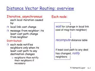
Iterative, asynchronous: each local iteration caused by: local link cost change DV update message from neighbor Distributed: each node notifies neighbors, but only when its DV changes neighbors then notify their neighbors if necessary wait for (change in local link cost or msg from neighbor) recompute estimates if DV to any dest has changed, notify neighbors Distance Vector Algorithm (5) Each node:
cost to x y z x 0 2 7 y from ∞ ∞ ∞ z ∞ ∞ ∞ 2 1 7 z x y Dx(y) = min{c(x,y) + Dy(y), c(x,z) + Dz(y)} = min{2+0, 7+1} = 2 Dx(z) = min{c(x,y) + Dy(z), c(x,z) + Dz(z)} = min{2+1, 7+0} = 3 node x table cost to x y z x 0 2 3 y from 2 0 1 z 7 1 0 node y table cost to x y z x ∞ ∞ ∞ 2 0 1 y from z ∞ ∞ ∞ node z table cost to x y z x ∞ ∞ ∞ y from ∞ ∞ ∞ z 7 1 0 time
cost to x y z x 0 2 7 y from ∞ ∞ ∞ z ∞ ∞ ∞ 2 1 7 z x y Dx(z) = min {c(x,y)+Dy(z), c(x,z)+Dz(z)} = min {2+1, 7+0} = 3 Dx(y) = min {c(x,y)+Dy(y), c(x,z)+Dz(y)} = min {2+0, 7+1} = 2 node x table cost to cost to x y z x y z x 0 2 3 x 0 2 3 y from 2 0 1 y from 2 0 1 z 7 1 0 z 3 1 0 node y table cost to cost to cost to x y z x y z x y z x ∞ ∞ x 0 2 7 ∞ 2 0 1 x 0 2 3 y y from 2 0 1 y from from 2 0 1 z z ∞ ∞ ∞ 7 1 0 z 3 1 0 node z table cost to cost to cost to x y z x y z x y z x 0 2 7 x 0 2 3 x ∞ ∞ ∞ y y 2 0 1 from from y 2 0 1 from ∞ ∞ ∞ z z z 3 1 0 3 1 0 7 1 0 time
Example 2Initial Distances to your neighbors 1 Distance to node B C Info at node A B C D E 7 0 7 ~ ~ 1 A 8 2 B A 7 0 1 ~ 8 C ~ 1 0 2 ~ 1 2 D ~ ~ 2 0 2 D E E 1 8 ~ 2 0
E Receives D’s Routes 1 Distance to node B C Info at node A B C D E 7 0 7 ~ ~ 1 A 8 2 B A 7 0 1 ~ 8 C ~ 1 0 2 ~ 1 2 D ~ ~ 2 0 2 D E E 1 8 ~ 2 0
E Updates Cost to C 1 Distance to node B C Info at node A B C D E 7 0 7 ~ ~ 1 A 8 2 B A 7 0 1 ~ 8 C ~ 1 0 2 ~ 1 2 D ~ ~ 2 0 2 D E E 1 8 4 2 0
A Receives B’s Routes 1 Distance to node B C Info at node A B C D E 7 0 7 ~ ~ 1 A 8 2 B A 7 0 1 ~ 8 C ~ 1 0 2 ~ 1 2 D ~ ~ 2 0 2 D E E 1 8 4 2 0
A Updates Cost to C 1 Distance to node B C Info at node A B C D E 7 0 7 8 ~ 1 A 8 2 B A 7 0 1 ~ 8 C ~ 1 0 2 ~ 1 2 D ~ ~ 2 0 2 D E E 1 8 4 2 0
A Receives E’s Routes 1 Distance to node B C Info at node A B C D E 7 0 7 8 ~ 1 A 8 2 B A 7 0 1 ~ 8 C ~ 1 0 2 ~ 1 2 D ~ ~ 2 0 2 D E E 1 8 4 2 0
A Updates Cost to C and D 1 Distance to node B C Info at node A B C D E 7 0 7 5 3 1 A 8 2 B A 7 0 1 ~ 8 C ~ 1 0 2 ~ 1 2 D ~ ~ 2 0 2 D E E 1 8 4 2 0
Final Distances 1 Distance to node B C Info at node A B C D E 7 0 6 5 3 1 A 8 2 B A 6 0 1 3 5 C 5 1 0 2 4 1 2 D 3 3 2 0 2 D E E 1 5 4 2 0
Final Distances After Link Failure 1 Distance to node B C Info at node A B C D E 7 0 7 8 10 1 A 8 2 B 7 0 1 3 8 A C 8 1 0 2 9 1 2 D 10 3 2 0 11 D E E 1 8 9 11 0
View From a Node E’s routing table 1 Next hop B C dest A B D 7 1 14 5 A B 8 2 7 8 5 A C 6 9 4 D 4 11 2 1 2 D E
The Bouncing Effect dest cost dest cost 1 A 1 A B B 1 C 1 C 2 1 25 C dest cost A 2 B 1
C Sends Routes to B dest cost dest cost A ~ A B B 1 C 1 C 2 1 25 C dest cost A 2 B 1
B Updates Distance to A dest cost dest cost A 3 A B B 1 C 1 C 2 1 25 C dest cost A 2 B 1
B Sends Routes to C dest cost dest cost A 3 A B B 1 C 1 C 2 1 25 C dest cost A 4 B 1
C Sends Routes to B dest cost dest cost A 5 A B B 1 C 1 C 2 1 25 C dest cost A 4 B 1
How Are These Loops Caused? • Observation 1: • B’s metric increases • Observation 2: • C picks B as next hop to A • But, the implicit path from C to A includes itself!
Solution 1: Holddowns • If metric increases, delay propagating information • in our example, B delays advertising route • C eventually thinks B’s route is gone, picks its own route • B then selects C as next hop • Adversely affects convergence
Other “Solutions” • Split horizon • B does not advertise route to C • Poisoned reverse • B advertises route to C with infinite distance Works for two node loops • does not work for loops with more nodes
A B 1 1 1 C 1 D Example Where Split Horizon Fails • When link breaks, C marks D as unreachable and reports that to A and B. • Suppose A learns it first. A now thinks best path to D is through B. A reports D unreachable to B and a route of cost=3 to C. • C thinks D is reachable through A at cost 4 and reports that to B. • B reports a cost 5 to A who reports new cost to C. • etc...
Avoiding the Bouncing Effect Select loop-free paths • One way of doing this: • each route advertisement carries entire path • if a router sees itself in path, it rejects the route BGP does it this way Space proportional to diameter Cheng, Riley et al
Distance Vector in Practice • RIP and RIP2 • uses split-horizon/poison reverse • BGP/IDRP • propagates entire path • path also used for effecting policies
LS vs. DV Algorithms The two algorithms take complimentary approaches: • Link State: Tell everyone what you know about your neighbors • Distance vector: Tell your neighbors what you know about everyone
Message complexity LS: with n nodes, E links, O(nE) msgs sent DV: exchange between neighbors only Speed of Convergence LS: O(n2) algorithm requires O(nE) msgs may have oscillations DV: convergence time varies may have routing loops count-to-infinity problem Robustness: what happens if router malfunctions? LS: node can advertise incorrect link cost each node computes only its own table DV: DV node can advertise incorrect path cost each node’s table used by others error propagates thru network Comparison of LS and DV Algorithms