Parametric Tests I & II
Parametric Tests I & II. January 31 and February 3, 2014. Note:. Some formulae are presented in this lecture to provide the general mathematical background to the topic or to demonstrate a concept. Do you need to know these formulae?. Recap: Vocabulary. Hypothesis


Parametric Tests I & II
E N D
Presentation Transcript
Parametric Tests I & II January 31 and February 3, 2014
Note: Some formulae are presented in this lecture to provide the general mathematical background to the topic or to demonstrate a concept. Do you need to know these formulae?
Recap: Vocabulary • Hypothesis • Statement of belief with respect to population values • Null • Hypothesis of no relationship • Alternative or research hypothesis • Test statistic • Like Z or t, used to determine the position of the mean in the hypothesized distribution of sample means • Critical region / critical value • The region at the far end of the distribution, also called the tail • One and two tailed tests • When Z or t fall within the critical region, or, are greater than the critical value, we reject the null hypothesis in favor of the alternative • The probability that a test statistic falls within the critical region (tail) is alpha. • Significance level • Alpha • Test of significance • Hypothesis test or the process of figuring out whether or not the test statistic falls within the critical region (and we reject the null) or below it (and we fail to reject the null)
Review: • One Sample Mean t test • Used to compare 1 sample mean with a population mean. • Average x from your sample compared to the population mean – a mean of “zero” • Confidence intervals • 95% / 99% • Allows us to calculate, with a specified degree of assurance, that the value of a population parameter such as mean, was captured • 1.96 and 2.54 +/- (s/sqrt n) • Confidence intervals give us a range that is sometimes very useful
Test Statistics Statistic = difference / measure of variability
t-Test: Paired and Independent Samples • Independent • Subjects in sample 1 have no connection to subjects in sample 2, such as comparing the BP of men to women. There should be no connection between the two groups. • Paired • There is a connection between scores in one group and scores in the other. • For example, comparing BP in a group of patients before and after a specific drug or lifestyle intervention. In this case, we can see that the changes in BP are connected between the pre and post measurements. • Calculations for paired and independent samples are different and yield different results • The paired t test calculation factors in an expected correlation between scores – based on this idea of connectedness • First step is always to determine if the samples are paired or independent.
Case Study: • Goal: • Evaluate the efficacy of a new antihypertensive medication • Research question: • Is the efficacy of the medication the same for males and females? • Is this a paired or independent sample? • Why? • Assumptions • Efficacy is measured as the mean change from baseline BP three months after taking the medication. • Data • BP is measured in mmHg.
Independent Samples t-test • Step 1 • State your hypothesis: • Research Hypothesis: • Mean SBP is higher in males than females • μ1 > μ2 or this could also be written as μ1 – μ2 > 0 • Null hypothesis: • Mean SBP is not higher in males than females • One or two tailed test? • μ1 ≤ μ2 or μ1 – μ2 ≤ 0 • Why? • Step 2 • Choose your significance level • Alpha 0.05 or perhaps 0.01
Independent Samples t-test • Step 3 • Compute t statistic using the following formula
Compute t Statistic • Step 4 • Given: • Mean 1 = 120.2 • Mean 2 = 108.2 • n1 and n2 = 15 • From the formula the pooled std deviation = 10.29 • So: • t = 120.2 – 108.2 - 0 / 10.29 [sqrt (1/15+1/15)] • t = 12 / 2.757 • t = 3.19
Step 4: Determine critical region From t statistic table, one tailed t-test, d.f.=(n1+n2)-2=28, critical value =1.70
Step 5: Test for significance • t statistic = 3.19 • This is within the critical region • This is greater than the critical value • So, we reject the null that • μ1 ≤ μ2 or μ1 –μ2 ≤0 at a p-value of <0.05 • How do we know P is < .05? • We know this because of the calculated and critical values. Because the calculated value is in the tail of the distribution, we know that P < .05.
Step 6: Confidence Interval • We can also calculate 95% confidence interval for this independent sample: • We use the same basic formula except now it reflects: • two sample means; degrees of freedom of 28 to be used to determine the critical value for t = .05; uses the pooled standard deviation • Mean difference is 12 • Critical value of t at 28 d.f. is 2.0484, alpha .05 (2 tailed) • Pooled s adjusted for sample size = 3.757 • So: • 12 +/- 2.0484(3.757) = 4.30 < u < 19.70 • This means we are 95% sure (or confident) that the population of males’ blood pressured ranges from a low of 4.3 points higher to as much as 19.7 points higher than females’ blood pressures
Inferences? • We now need to draw meaningful conclusions that are supported by our statistical analyses • SBP of males is significantly greater than the SBP of females or • SBP of females is significantly lower than the SBP of males • What if I had to do several, say 10 of these t-tests to get my answer? What kind of error increases?
Case Two: Paired Samples t Test • Using the same data as Case One, we can now try to determine whether the experimental conditions led to change in blood pressure. • In a paired sample test, each subject in the treatment group will be used as its own control. • This has the benefit of reducing some kinds of experimental error since variability due to extraneous factors is reduced. • We will also have fewer degrees of freedom since we will have only 1 sample, but with two observations • When calculating a paired t - n always equals the number of pairs • With fewer d.f. all else equal, the t will be larger, and so the confidence interval will be larger. • One other issue: do we analyze just males or do we include females in this analysis too? Pro’s? Con’s?
Case Two: Paired Samples t Test • Step 1 • Hypothesis (H1): SBP is lower in males after taking new medication • μ1 ≠ μ2 or μ1 – μ2 ≠ 0 • Null hypothesis (H0): SBP is not higher in males than females • μ1 = μ2 or μ1 – μ2 = 0 • We will use a two-tailed test since we don’t know if the SBP will be higher or lower
Paired Samples t test • Step 2 • Significant level: • α=0.05 • Step 3 • Compute t statistic using the following formula: (next slide)
NOTE: • - d is the mean difference between x (before) and y (after) • Sd is the estimate of the standard deviation of the differences • n is always the number of pairs
Determine Critical Region From t statistic table, two tailed t-test, d.f.= n-1 = 14, critical value =2.1448
Test for Significance • Calculate t • -0.80 / (3.43/sqrt 15) = -0.90 • Because t statistic = -0.90 and it falls outside the critical region, which means it is less than the critical value of +/- 2.1448 we fail to reject the null hypothesis of no difference • This means there is no difference in SBP between the pre and post measurements on these paired differences. • What would we report as the P value? Why? • Next, we could calc the 95% confidence interval: • (120.2 – 121.0 ) +/- t (0.885) • = -0.80 +/- 2.145 (.0885) • = −2.70 < u < 1.10 • So, our range is -2.70 < u1 – u2 < 1.10 • What does this confidence interval mean? What is the significance of the fact that zero is contained within the interval? Does this support our conclusion based on the test statistic?
Determination of Sample Size • How large a sample size do I need to obtain a statistically meaningful result? • Factors to be considered: • How much error can I live with in estimating the population mean? • What level of confidence do we need? • How much variability exists in the data?
Determining Sample Size Sample size can be calculated by rearranging the formula for Z statistic
Case Study 3 • You want to estimate the cholesterol level of a population within 10mg/dl. You know that σ=20 and you want to stay within 95% confidence that x is within 10 units of μ. • Sample size = (1.96)(20)/10=15.36 • Note: 1.96 comes from the Z statistic table corresponding to 95% confidence • If you don’t know σ, use s as an estimate and then use the t distribution for your values
Parametric Tests II February 3, 2014
Review • True or False: • Increasing sample size will always improve a study. • The desired alpha level, the variability in the population and the size of the difference that is being measured are used to estimate sample size. • Very good results can sometimes be obtained with very small samples. • Increasing the alpha level from 0.05 to 0.1 will decrease the estimated size of the sample needed for a study.
Review • True or False • t-tests are used to compare means or averages in a population. • Comparing the SBP of men to women is an example of a dependent sample t-test. • What would be one impact of doing 7 t-tests for multiple means in a study of SBP? (Multi-choice) • You would have a better chance of finding significant results. • You would have a lot less work to do than if you were doing only 1 t-test. • You would increase the chances that you found one of the “5” times in 100 that you got your results by chance alone, and not because there is a real difference in the sample means. • Your patients arms would hurt from all the blood pressure measurements.
Review • True or False • Statistical power is defined as 1-beta error (type II error). • Statistical power is the probability of getting the right answer (e.g., rejecting the null hypothesis when its false). • Statistical power stems from knowing statistics better than others you work with. • One can think of statistical power as your “confidence” in your results. • Power is 1 – the chance you got it wrong = the probability you got it right. • For most studies researchers plan to set at Alpha 0.05, Beta 0.20, and Power at 80% • While alpha = 0.05 is an absolute according to most statistical experts, power is not, in other words there is not rock solid cut-off. • Power analysis is used in sample size planning and can be used for hypothesis testing. • To calculate power you need to know: your desired alpha level, an estimate of how big the effect is in the population, (like the standardized difference between two means) and an estimate of the variability.
What we need to do today: Develop an understanding of how we compare means when we have multiple groups. Discuss the concepts of within between groups differences and between groups differences. Learn how to interpret an analysis of variance model Understand the concept of “range tests” or “multiple comparisons”
Analysis of Variance • ANOVA • Allows comparison of data from three or more independent groups • Suppose we have 3 groups of patients • Children < 18 • Adults 19-64 • Seniors > 65 • And, we want to know if the BP of these three groups are significantly different • We could do several t tests and use logic to conclude what we want to know • Increases experiment-wise error by repeated t-tests • Null hypothesis: • μ1 = μ2 = μ3or μ1 – μ2 – μ3 = 0 • K is the number of groups which in this case is 3 • (t-tests are just to compare one mean against another) • Alternative hypothesis: • At least one of the means μ is not equal to the others
Why do an ANOVA? This procedure offers us a way to do multiple tests between groups while controlling for the error introduced by multiple tests. The more times you perform a test, the more likely you are to find one of those pesky 5 times in 100 that you got your answer by chance alone.
Assumptions of ANOVA • Observations are independent • as in independent t-test • Observations in each group are normally distributed • In other words, they would have a bell shaped curve • Variances of each of the groups is homogeneous • Each group has about the same variance • Note: • ANOVA is rather robust • This means, in statistical terms, that ANOVA is relatively insensitive to violations of normality and homogeneity assumptions as long as the sample size is large and nearly equal for each group • ANOVA is perfect for mean comparisons with N> 25 per group; • Have done it with as few as 6 for one pharmacologist!
General Idea of ANOVA • Goal • To find out if there is a difference between our three group means: children, adults and seniors. • How? • Use a test statistic that will somehow compare the means of these three groups • F Statistic = between groups variance / within groups variance • There are F tables just like t and Z • Computationally, F = mean square between / mean square within • If the between-group variance is enough bigger than the within-group variance there will be significant differences
Key Feature of ANOVA • Variance has two components: • Variance within groups (d.f.= N- k) • Variance between groups (d.f. = k -1) • These two variance estimates are used to calculate the F statistic
Hypothesis Testing using ANOVA • 3 main steps • State your hypotheses • Calculate F test statistic • Determine critical region based on α and reject the null hypothesis if the F statistic is greater than critical value
Case Study • Question: Is there a significant difference in weight gain among the children fed four different brands of cereal? • Step 1 • Alternative H1: One or more of the means are different from the others • Null: μ1 = μ2 = μ3 = μ4 (no differences in means)
Data • Weight gain of children fed on four different brands of cereal (N=20, 5 children per group) • Does this data look like there will be a difference between the group means?
Have your computer calculate the F statistic, which is the ratio of the between to within groups variance – you will get a table that looks like this:
ANOVA Table • From F statistic distribution, critical value of α=0.05 for F3,16=3.24 (our F was over 7) • Because calculated F statistic is >3.24 and falls within the critical region, we reject H0 • Conclusion: • There is a significant difference in weight gain among the children that were fed the four different brands of cereal
But: Which Means are Significantly Different? ANOVA only tells us that there is a difference between all the means. Multiple t tests between the various pairs of means are not appropriate because the probability of incorrectly rejecting the hypothesis increases with the number of t-tests performed
Which Means are SignificantlyDifferent? • Must use a post-hoc test to find out which of the means is (are) different • This is called a multiple comparisons test. • Some examples are: • Tukey • Tukey-Kramer • Scheffe • Bonferroni • Dunnett’s
Tukey’s Test Uses a formula to determine mathematically if each mean difference is greater than an anticipated critical value calculated like a test statistic. This procedure identifies which means are actually different from each other. In our example, this is 3.73, so we compare each pair of mean differences to this number, if the difference is greater than 3.73 we know that those two means are different