NOAO LSST Science Working Group

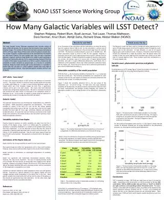
1. NOAO LSST Science Working Group How Many Galactic Variables will LSST Detect? Stephen Ridgway, Robert Blum, Buell Jannuzi, Tod Lauer, Thomas Matheson, Dara Norman, Knut Olsen, AbhijitSaha, Richard Shaw, Alistair Walker (NOAO) Abstract The Large Synoptic Survey Telescope operational plan includes release of alerts, within 60 seconds, for all sources that are found to have varied from template images. The number of these alerts has been variously estimated at 10^5 to 10^6 per night. Many of these alerts will be for galactic variable stars. The number of galactic variables detected can be estimated from the bottom up, with known statistics for each variable type. Here we take a top-down approach. A galactic synthesis model (Robin et al, 2003) is used to generate a fictitious but statistically valid star list for a given pointing. Analysis of the first 3 months of the Kepler survey (Ciardi et al, 2011) is used to characterize the probability of stellar variability by spectral type, as a function of variability amplitude. With this model and the LSST survey parameters, it is possible to predict that LSST will alert on ~2X10^5 galactic variable stars each night at intermediate galactic latitude. Most detected galactic variables will be K and M dwarfs. Results for one field As an illustration of the calculation and the implications, we show the results here for a galactic field at l=96, b=-60. For the calculation, a surface area of 10 square degrees was adopted (just a few percent larger than the nominal LSST FOV). The Besancon model produced a source list of 105,982 stars. We adopt parameters similar to those of LSST for this example. Imposing a saturation limit of g=15 and 5-sigma photon limit of g=24.7 reduces the star list to 65,306 targets. In determining which variables to classify as detectable, we consider the photon noise of a source with a 5-sigma photon-limited detection, and with a 5-sigma differential photometry cutoff (here, this is effectively a free parameter, which may reflect systematic calibration limits, PSF mis-match, etc). These two error sources were combined quadratically to give a level of detectable variability, s0. Detectable variability of the model population With this level, s0, the fractional probability of variation for s > s0is computed from the function f(s). The fractional probabilities are computed for each member of the star list, and subsets of interest are summed to determine the predicted total number of variables detectable. Figure 1 shows the variability detection limit s0 for two values of the photometry cut – 10 and 25 mmag. For faint stars, only large amplitude variability will be detected, and photon statistics dominate the detection limit for these. Consequently, and perhaps counter-intuitively, the number of detectable variables is not a strong function of the differential photometry cut. Trends across the sky The Besancon model has been used to simulate the stellar populations for a series of fields along a great circle from the galactic center through the south galactic pole to the anticenter. At high latitudes, an area of 10 square degrees gave useful statistical results. However, it should be noted that these models are computed for a single sky position. Near the galactic plane, the number of stars was quite large and the simulation was carried out for field sizes of 1 square degree or less. These numbers were then normalized to a 10 square degree area. s0 Variable count, photometric precision and galactic latitude For photometry cut of 50 mmag, Figure 2 shows the variation of number of detectable variables per 10 sq-deg field with galactic latitude. LSST alerts - how many? A major and important product of LSST will the the detection of transient sources. The project intends to announce these quickly (within 60 seconds) to enable rapid follow-up. In order to avoid missing significant events, all targets which vary from template images by more than a significance criterion will be put in the alert stream. This means that most detected variable stars will generate repeated alerts. We wish to estimate the volume and content of this alert stream, as discussed in the companion poster (T. Matheson et al.). In this poster we explain a simple empirical approach to estimating the number of variable stars that LSST will detect. Galactic model The approach reported here uses the Besancon model (Robin et al, 2003) for the galactic stellar population composition and distribution. This model provides its output in the form of a star list for the chosen galactic coordinates and surface area on the sky. For each star in the list, the model provides the basic data for mass, age, luminosity, distance and apparent (reddened) colors. Of course the stars are fictitious, but thanks to the model design and constraints, the model produces star lists which reproduce major observed population statistics. Variability statistics from Kepler Empirical data for statistics on stellar variability are taken from the first 3 months of the Kepler survey. Ciardi et al (2011) give the probability of variability vs variability amplitude in a number of bins greater than and less than 0.01 magnitudes. It can be observed in these data that the trend of probability is approximately described with a function of the form f(s) = bs-a, where s is the variability amplitude. Data for each major spectral type has been fit with such a function. The exponent a is found to fall in the range a = 1.3 to 1.8. Limitations of the Kepler data set Kepler statistics for strong variability are weak for most spectral types. Rare spectral types are either not represented at all or have small numbers. However, these sources will have little impact on the count of total variables. Kepler provides no information on wavelength dependence of variability amplitude. Kepler has significant and imprecisely documented selection effects. However, this may not be important. The case of eclipsing binaries stands out as perhaps the most serious, as known EB’s were singled out for special handling. However, an analsyis of Kepler EB’s (Prsa et al, 2011) finds that only 18% of the Kepler-identified EB’s were previously known, and an uncertainty of this magnitude is acceptable to our study. Variable star statistics depend on stellar population, hence vary with galactic latitude. Centered on a galactic latitude of 13.5 degrees, Kepler will more strongly represent stellar populations in the plane than in the halo. Most galactic variable stars detected by LSST will be near the plane of the galaxy, so this should not significantly bias total detections. On the other hand, high latitude fields will be less accurately described. 106 Detected variables per 10 sq-deg 104 102 Angle Figure 2. The total number of detectable variables in a 10 sq deg field, with a photometric precision cutoff of 0.05 mag. The angle is along the arc of a great circle from the galactic center through the south pole to the anticenter. The dip at 0 degrees is due to extinction in the plane. For the vicinity of the galactic pole and (l,b = 0,-20), Figure 3 shows how the number of detected variables per 10 sq-deg depends on the photometric precision cut, showing the realtively weak dependence. g-magnitude Figure 1. The smallest detectable fractional variability as a function of g-magnitude, for differential photometry cut of 10 and 25 mmag. Table 1 shows the distribution of expected variability among spectral types for the model population, the Kepler statistics, and the expected LSST sensitivity. The absence of giants and A dwarfs results from the brightness cutoff due to detector saturation, assumed here to be at g=15. Detected variables per 10 sq-deg Variability amplitude limit (mmag) Figure 3. The total number of detectable variables in a 10 sq deg fields, one near the galactic pole and one near (l,b = 0,-20), as it depends on the differential photometry cut. In each visit to a field, only some of the variable stars will be detectably different from a reference template. Conclusions LSST is expected to image ~400 fields per night (most at least 2x during the night). Depending on the photometric cut and the position on the sky, LSST could detect ~500 to 20000 variable stars per field, or ~2x10^5 to 8X10^6 per night, and issue a corresponding number of transient alerts. The higher numbers, associated with the galactic plane, are unlikely to be realized as the typical separation between variables will be ~2 arcsec, and crowding will require that the cut for detected variation be set somewhat higher. Most variables stars (~90%) will be K and M dwarfs, readily identified as such from photometry. Table 1. The predicted number of detectable variables in a 10 Sq Deg field at l=96, b=-60, in the g-filter. References Ciardi et al, 2011, AJ 141, 108. Prsa, Pepper and Stassun, 2011, AJ 142, 52. Robin et al, 2003, A&A 409, 523. In this field, it is estimated that at a 25 mmag cut, 1.2% of galactic stars detected by LSST will have variability detectable between maximum and minimum brightness. Approximately half of detectable variables will be found to have varied from a template image at an arbitrary epoch.