Linear Programming
Linear Programming. Introduction. Mathematical programming is used to find the best or optimal solution to a problem that requires a decision or set of decisions about how best to use a set of limited resources to achieve a state goal of objectives. Steps involved in mathematical programming

Linear Programming
E N D
Presentation Transcript
Linear Programming Dr.G.Suresh Kumar@KL University
Introduction • Mathematical programming is used to find the best or optimal solution to a problem that requires a decision or set of decisions about how best to use a set of limited resources to achieve a state goal of objectives. • Steps involved in mathematical programming • Conversion of stated problem into a mathematical model that abstracts all the essential elements of the problem. • Exploration of different solutions of the problem. • Finding out the most suitable or optimum solution. • Linear programming requires that all the mathematical functions in the model be linear functions. Dr.G.Suresh Kumar@KL University
General LPP Max/min Z = c1x1 + c2x2 + ... + cnxn subject to: a11x1 + a12x2 + ... + a1nxn (≤, =, ≥) b1 a21x1 + a22x2 + ... + a2nxn (≤, =, ≥) b2 : am1x1 + am2x2 + ... + amnxn (≤, =, ≥) bm and xj ≥ 0, j = 1, 2, 3, …, n. xj = decision variables bi = constraint levels cj = objective function coefficients aij = constraint coefficients Dr.G.Suresh Kumar@KL University
Formation of LPP • A manufacturer produces two types of models M1 and M2. Each M1 model requires 4 hours of grinding and 2 hours of polishing; whereas M2 model requires 2 hours of grinding and 5 hours of polishing. The manufacturer has 2 grinders and 3 polishers. Each grinder works for 40 hours a week and each polisher works for 60 hours a week. Profit on an M1 model is Rs. 3 and on M2 model is Rs. 4. Whatever is produced in a week is sold in the market. How should the manufacturer allocate his production capacity to the two types of models so that he make the maximum profit in a week. Dr.G.Suresh Kumar@KL University
Solution • Let x be the number of M1 models and y be the number of M2 models produced in a week. • Then the weekly profit is Z = 3x + 4y. • The total number of grinding hours needed in a week to produce x and y is 4x + 2y. • The total number of polishing hours needed in a week to produce x and y is 2x + 5y. Dr.G.Suresh Kumar@KL University
Solution cont… • Since the number of grinding hours is not more than 80 and the number of polishing hours not more than 180, therefore 4x + 2y ≤ 80 2x + 5y ≤ 180. • Also, the negative number of models are not produced, we must have x ≥ 0 and y ≥ 0. Dr.G.Suresh Kumar@KL University
Solution cont… • Now the problem is to find x, y which Maximize Z = 3x + 4y Subject to 4x + 2y ≤ 80 2x + 5y ≤ 180 and x, y ≥ 0. Dr.G.Suresh Kumar@KL University
Problem#2 • An aeroplane can carry a maximum of 200 passengers. A profit of Rs.400 is made on each first class ticket and a profit of Rs. 300 is made on each economy class ticket. The airline reserves at least 20 seats for first class. However, at least 4 times as many passengers prefer to travel by economy class than by the first class. How many tickets of each class must be sold in order to maximize profit for the airline ? Formulate the problem as L.P. model and then solve. Dr.G.Suresh Kumar@KL University
Solution • Maximize Z = 400x + 300y subject to x + y ≤ 200 x ≥ 20 y ≥ 4x and x, y ≥ 0. Dr.G.Suresh Kumar@KL University
Problem#3 • Consider the following problem faced by a production planner in a soft-drink plant. He has two bottling machines A and B. A is designed for 8-ounce bottles and B for 16-ounce bottles. However, each can be used on both types with some loss of efficiency. The following data is available : Machine 8-ounce bottle 16-ounce bottle A 100/ minute 40/ minute B 60/ minute 75/ minute Dr.G.Suresh Kumar@KL University
Problem#3 The machines can be run 8 hours per day, 5 days per week. Profit on 8-ounce bottle is 15 paise and on a 16-ounce bottle is 25 paise. Weekly production of the drink cannot exceed 300,000 ounces and the market can absorb 25,000 8-ounce bottles and 7,000 16-ounce bottles per week. The planner wishes to maximize his profit subject to all production and marketing restrictions. Formulate the problem as L.P model. Dr.G.Suresh Kumar@KL University
Solution • Maximize Z = 0.15x+0.25y subject to 2x + 5y ≤ 480,000 5x + 4y ≤ 720,000 8x + 16y ≤ 300,000 x ≤ 25, 000 y ≤ 7,000 and x, y ≥ 0. Dr.G.Suresh Kumar@KL University
General LPP Max/min Z = c1x1 + c2x2 + ... + cnxn subject to: a11x1 + a12x2 + ... + a1nxn (≤, =, ≥) b1 a21x1 + a22x2 + ... + a2nxn (≤, =, ≥) b2 : am1x1 + am2x2 + ... + amnxn (≤, =, ≥) bm xj = decision variables bi = constraint levels cj = objective function coefficients aij = constraint coefficients Dr.G.Suresh Kumar@KL University
Solutions of LPP • A set of values x1, x2, …, xn which satisfies the constraints of LPP is called its solution. • Any solution to a LPP which satisfies the non-negativity restrictions is called its feasible solution. • Any feasible solution which maximizes or minimizes the objective function is called its optimal solution. Dr.G.Suresh Kumar@KL University
Solutions of LPP • A solution is obtained by setting n-m variables to zero (if m equality constraints and n variables of LPP) is called a basic solution. • Basic solution of LPP is also satisfies the non-negativity restrictions is called basic feasible solution. • Basic feasible solution which maximizes or minimizes the objective function is called its optimal solution. • A basic feasible solution in which all basic variable are non-zero is called a non-degenerate basic feasible solution otherwise it is a degenerate basic feasible solution. Dr.G.Suresh Kumar@KL University
Problem#1 • Find all the basic solutions of the following system of equations identifying in each case the basic and non-basic variables. 2x1 + x2 + 4x3 = 11 3x1 + x2 + 5x3 = 14 Ans : (3, 5, 0) basic x1, x2 non-basic x3. (0, 3, -1) basic x2, x3 non-basic x1. (1/2, 0, 5/2) basic x1, x3 non-basic x2. Dr.G.Suresh Kumar@KL University
Problem#2 • Find an optimal solution to the following LPP by computing all basic solutions and then finding one that maximizes objective function. Max. Z = 2x1 + 3x2 + 4x3 + 7x4 Subject to 2x1 + 3x2 - x3 + 4x4 = 8 x1 - 2x2 + 6x3 -7x4 = -3 and x1, x2, x3, x4 ≥ 0. Ans : (0, 0, 44/17, 45/17) and Z=28.9 Dr.G.Suresh Kumar@KL University
Slack variables • If the constraints of a general LPP be ai1x1 + ai2x2 + ... + ainxn ≤ bi (i = 1, 2,…), then the non-negative variables si which satisfy ai1x1 + ai2x2 + ... + ainxn + si = bi (i = 1, 2,…) are called slack variables. Dr.G.Suresh Kumar@KL University
Surplus variables • If the constraints of a general LPP be ai1x1 + ai2x2 + ... + ainxn ≥ bi (i = 1, 2,…), then the non-negative variables si which satisfy ai1x1 + ai2x2 + ... + ainxn - si = bi (i = 1, 2,…) are called surplus variables. Dr.G.Suresh Kumar@KL University
Canonical form of LPP The canonical form of LPP has • Objective function is of maximization type. • All constraints are of ≤ type. • All variables are non-negative. Dr.G.Suresh Kumar@KL University
Standard form of LPP The standard form of LPP has • Objective function is of maximization type • All constraints are expressed as equations • Right hand side of each constraint is non-negative • All variables are non-negative. Dr.G.Suresh Kumar@KL University
Simplex Method • Step#1: (i) Check whether the objective function is to be maximized or minimized. If minimized, then convert it into maximization using Min. Z = - Max. (-Z). (ii) Check whether all b’s are positive. If negative, then multiply by ‘-1’ both sides of the corresponding constraint. Dr.G.Suresh Kumar@KL University
Simplex Method Step#2: Express the problem in the standard form. Convert all inequalities into equations by introducing slack or surplus variables in the constraints of the LPP. Step#3 : Find an initial basic feasible solution and form the initial simplex table. Dr.G.Suresh Kumar@KL University
Initial Simplex Table cj c1 c2 … cn 0 0 … 0 Mini CB xB values a1 a2 … an an+1 an+2 … an+m ratio 0 s1 b1 a11 a12 … a1n 1 0 … 0 0 s2 b2 a21 a22 … a2n 0 1 … 0 … … …. … … … … … … … … 0 sm bm am1 am2 … amn 0 0 … 1 Zj-cj -c1 -c2 … -cn 0 0 … 0 Dr.G.Suresh Kumar@KL University
Simplex Method Step#4 : Optimality test Compute Zj-cj, where Zj = ∑ cBiaij. If all Zj-cj ≥ 0, then the current basic feasible solutions is optimal. If even one Zj-cj < 0, then the current basic feasible solution is not optimal and proceed to the next step. Dr.G.Suresh Kumar@KL University
Simplex Method Step#5: (i) identifying incoming vector Compute Zk-ck = Min. {Zj-cj/ Zj-cj < 0}, then ak is the entering(incoming) vector. If there is a tie select any one. (ii) identifying outgoing vector Compute Min.{xBi/aik, aik > 0} = xBr/ark, then ar is the out going vector. The element ark is called key element. If all aik≤0, then the problem has an unbounded solution and we stop the process. Dr.G.Suresh Kumar@KL University
Simplex Method (iii) iterate towards an optimal solution Covert the key element to unity by dividing the key row by the key element. Then make all other elements of the key column zero by subtracting proper multiples of key row from other rows. Step#6 : Go to step#4 and repeat the procedure until either an optimal solution or an unbounded solution is obtained. Dr.G.Suresh Kumar@KL University
Problem#1 Maximize Z = 5x1 + 3x2 Subject to x1 + x2 ≤ 2 5x1 + 2x2 ≤ 10 3x1 + 8x2 ≤ 12 and x1, x2 ≥ 0. Dr.G.Suresh Kumar@KL University
Solution • In standard form Maximize Z = 5x1 + 3x2+0s1+0s2+0s3 Subject to x1 + x2 +s1 +0s2 +0s3= 2 5x1 + 2x2 +0s1+s2 +0s3=10 3x1 + 8x2 +0s1 +0s2+s3= 12 and x1, x2 , s1, s2, s3≥ 0. Dr.G.Suresh Kumar@KL University
Initial Simplex Table cj 5 3 0 0 0 Mini CB xB values a1 a2 a3 a4 a5 ratio 0 s1 2 1 1 1 0 0 2 0 s2 10 5 2 0 1 0 2 0 s3 12 3 8 0 0 1 4 Zj-cj -5 -3 0 0 0 1 Dr.G.Suresh Kumar@KL University
First Simplex Table cj 5 3 0 0 0 Mini CB xB values a1 a2 a3 a4 a5 ratio 5 x1 2 1 1 1 0 0 0 s2 0 0 -3 -5 1 0 0 s3 6 0 5 -3 0 1 Zj-cj 0 2 5 0 0 Dr.G.Suresh Kumar@KL University
Solution • Since all Zj-cj ≥ 0, the current basic feasible solution is optimal. • Therefore the optimal solution to the given problem is x1= 2, x2 = 0 and maximum Z= 5(2)+3(0)=10. Dr.G.Suresh Kumar@KL University
Problem#2 Minimize Z = x1 - 3x2 + 3x3 Subject to 3x1 - x2+ 2x3 ≤ 7 2x1 + 4x2 ≥ -12 -4x1 + 3x2 + 8x3≤ 10 and x1, x2, x3 ≥ 0. Dr.G.Suresh Kumar@KL University
Solution • In standard form Maximize Zʹ = -x1+3x2 -3x3+0s1+0s2+0s3 Subject to 3x1 - x2 +2x3+s1 +0s2 +0s3= 7 -2x1 - 4x2+0x3+0s1+s2 +0s3=12 -4x1 + 3x2+8x3+0s1 +0s2+s3= 10 and x1, x2, x3, s1, s2, s3≥ 0. Dr.G.Suresh Kumar@KL University
Initial Simplex Table cj -1 3 -3 0 0 0 Mini CB xB values a1 a2 a3 a4 a5 a6 ratio 0 s1 7 3 -1 2 1 0 0 -- 0 s2 12 -2 -4 0 0 1 0 -- 0 s3 10 -4 3 8 0 0 1 10/3 Zj-cj 1 -3 3 0 0 0 3 Dr.G.Suresh Kumar@KL University
Improved Simplex Table-I cj -1 3 -3 0 0 0 Mini CB xB values a1 a2 a3 a4 a5 a6 ratio 0 s1 31/3 5/3 0 14/3 1 0 1/3 31/5 0 s2 76/3 -22/3 0 32/3 0 1 4/3 -- 3 x2 10/3 -4/3 1 8/3 0 0 1/3 -- Zj-cj -3 0 11 0 0 1 5/3 Dr.G.Suresh Kumar@KL University
Improved Simplex Table-II cj -1 3 -3 0 0 0 Mini CB xB values a1 a2 a3 a4 a5 a6 ratio -1 x1 31/5 1 0 14/5 3/5 0 1/5 0 s2 352/5 0 0 156/5 22/5 1 14/5 3 x2 58/5 0 1 32/5 4/5 0 3/5 Zj-cj 0 0 82/5 9/5 0 8/5 Dr.G.Suresh Kumar@KL University
Solution • Since all Zj-cj ≥ 0, the current basic feasible solution is optimal. • Therefore the optimal solution to the given problem is x1= 31/5, x2 = 58/5, x3=0 and maximum Zʹ= -1(31/5)+3(58/5)-3(0)=143/5. Minimum Z = -(Max.Zʹ) = -143/5 Dr.G.Suresh Kumar@KL University
Problem#3 • A farmer has 1,000 acres of land on which he can grow corn, wheat or soya-bean. Each acre of corn costs Rs. 100 for preparation, requires 7 man-days of work and yields a profit of Rs. 30. An acre of wheat costs Rs. 120 for preparation, requires 10 man-days of work and yields a profit of Rs. 40. An acre of soya-beans costs Rs. 70 for preparation, requires 8 man-days of work and yields a profit of Rs. 20. If the farmer has Rs. 100,000 for preparation and can count on 8,000 man-days of work, how many acres should be allocated to each crop to maximize profit? Dr.G.Suresh Kumar@KL University
Solution Let x, y, z be the number of acres of corn, wheat, soy-bean respectively. Then the given problem in LPP model: Maximize Z = 30x + 40y + 20z Subject to 100x +120y+70z ≤ 1,00,000 7x + 10y + 8z ≤ 8,000 x + y + z ≤ 1000 and x, y, z ≥ 0. Ans: x = 250, y = 625, z = 0. Dr.G.Suresh Kumar@KL University
Initial Simplex Table cj 30 40 20 0 0 0 Mini CB xB values a1 a2 a3 a4 a5 a6 ratio 0 s1 10000 100 12 7 1 0 0 833.3 0 s2 8000 7 10 8 0 1 0 800 0 s3 1000 1 1 1 0 0 1 1000 Zj-cj -30 -40 -20 0 0 0 Dr.G.Suresh Kumar@KL University
Improved Initial Simplex Table cj 30 40 20 0 0 0 Mini CB xB values a1 a2 a3 a4 a5 a6 ratio 0 s1 4000 16 0 -26 1 -12 0 250 40 x2 800 7/10 1 8/10 0 1/10 0 1142 0 s3 200 3/10 0 1/5 0 -1/10 1 666.6 Zj-cj -2 0 12 0 4 0 Dr.G.Suresh Kumar@KL University
Improved Initial Simplex Table cj 30 40 20 0 0 0 Mini CB xB values a1 a2 a3 a4 a5 a6 ratio 30 x1 250 1 0 -13/8 1/16 -3/4 0 40 x2 625 0 1 31/16 -7/16 5/8 0 0 s3 125 0 0 11/16 -3/16 1/8 1 Zj-cj 0 0 5/2 1/8 5/2 0 Dr.G.Suresh Kumar@KL University
Solution • Since all Zj-cj ≥ 0, the current basic feasible solution is optimal. • Therefore the optimal solution to the given problem is x1= 250, x2 = 625, x3=0 and Maximum Z= 30(250)+40(625)+20(0) = 32500 Dr.G.Suresh Kumar@KL University
Problem#4 • A firm produces three products which are processed on three machines. The relevant data is given below Dr.G.Suresh Kumar@KL University
Problem#4 The profit per unit for product A, B and C is Rs. 4, Rs. 3 and Rs.6 respectively. Determine the daily number of units to be manufactured for each product. Assume that all the units produced are consumed in the market. Dr.G.Suresh Kumar@KL University
Solution Let x1, x2, x3 be the number of units of Products A, B, C to be produced, then the problem in LP model Maximize Z = 4x1 + 3x2 + 6x3 Subject to 2x1 + 3x2+ 2x3 ≤ 440 4x1 + 3x3 ≤ 470 2x1 + 5x2 ≤ 430 and x1, x2, x3 ≥ 0. The optimal solution x1=0, x2=380/9, x3=470/3 and Zmax= 1066.67 rupees. Dr.G.Suresh Kumar@KL University
Artificial variable Techniques • Big M-Method or Method of Penalties : Step#1: Express the problem in standard form Step#2: Add non-negative variable to the left hand side of all constraints which are of (≥) or (=) type. Such new variables are called artificial variables. The penalty or cost for these variables in the objective function is –M, M>0 and large. Dr.G.Suresh Kumar@KL University
Big M-Method (Charne’s Penalty) Step#3 : solve the modified LPP by simplex method. At any iteration of the simplex method, one of the following three cases may arise: Case(i) There remains no artificial variable in the basis and the optimality condition satisfied. Then the solution is optimal solution. Dr.G.Suresh Kumar@KL University

