models: reinforcement learning & fMRI

models: reinforcement learning & fMRI Nathaniel Daw 11/28/2007

overview • reinforcement learning • model fitting: behavior • model fitting: fMRI

overview • reinforcement learning • simple example • tracking • choice • model fitting: behavior • model fitting: fMRI

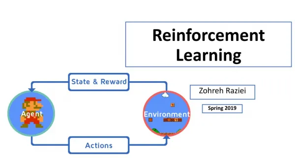
Reinforcement learning: the problem Optimal choice learned by repeated trial-and-error • eg between slot machines that pay off with different probabilities But… • Payoff amounts & probabilities may be unknown • May additionally be changing • Decisions may be sequentially structured (chess, mazes: this we wont consider today) Very hard computational problem; computational shortcuts essential Interplay between what you can and should do Both have behavioral & neural consequences

Simple example n-armed bandit, unknown but IID payoffs • surprisingly rich problem Vague strategy to maximize expected payoff: • Predict expected payoff for each option • Choose the best (?) • Learn from outcome to improve predictions

Simple example • Predict expected payoff for each option • Take VL = last reward received on option L • (more generally, some weighted average of past rewards) • This is an unbiased, albeit lousy, estimator • Choose the best • (more generally, choose stochastically s.t. the machine judged richer is more likely to be chosen) Say left machine pays 10 with prob 10%, 0 owise Say right machine pays 1 always What happens? (Niv et al. 2000; Bateson & Kacelnik)

Behavioral anomalies • Apparent risk aversion arises due to learning, i.e. due to the way payoffs are estimated • Even though we are trying to optimize expected reward, risk neutral • Easy to construct other examples for risk proneness, “probability matching” • Behavioral anomalies can have computational roots • Sampling and choice interact in subtle ways

what can we do?

Reward prediction weight What can we do? Exponentially weighted running average of rewards on an option: trials into past Convenient form because it can be recursively maintained (‘exponential filter’) ‘error-driven learning’, ‘delta rule’, ‘Rescorla-Wagner’

what should we do? [learning]

Bayesian view Specify ‘generative model’ for payoffs • Assume payoff following choice of A is Gaussian with unknown mean mA; known variance s2PAYOFF • Assume mean mA changes via a Gaussian random walk with zero mean and variance s2WALK payoff for A mA trials

Bayesian view Describe prior beliefs about parameters as a probability distribution • Assume they are Gaussian with mean ; variance Update beliefs in light of experience with Bayes’ rule mean of payoff for A P(mA | payoff) /P(payoff | mA)P(mA)

Bayesian belief updating mean of payoff for A

Notes on Kalman filter • Looks like Rescorla/Wagner but • We track uncertainty as well as mean • Learning rate is function of uncertainty (asymptotically constant but nonzero) • Why do we exponentially weight past rewards?

what should we do? [choice]

The n-armed bandit n slot machines binary payoffs, unknown fixed probabilities you get some limited (technically: random, exponentially distributed) number of spins want to maximize income surprisingly rich problem

The n-armed bandit • Track payoff probabilities Bayesian: learn a distributionover possible probs for each machine This is easy: Just requires counting wins and losses (Beta posterior)

The n-armed bandit 2. Choose This is hard. Why?

The explore-exploit dilemma 2. Choose Simply choosing apparently best machine might miss something better: must balance exploration and exploitation simple heuristics, eg choose at random once in a while

Explore / exploit Which should you choose? left bandit: 4/8 spins rewarded right bandit: 1/2 spins rewarded mean of both distributions: 50%

Explore / exploit Which should you choose? left bandit: 4/8 spins rewarded right bandit: 1/2 spins rewarded green bandit more uncertain (distribution has larger variance)

Explore / exploit although green bandit has a larger chance of being worse… Which should you choose? Trade off uncertainty, exp value, horizon ‘Value of information’: exploring improves future choices How to quantify? … it also has a larger chance of being better …which would be useful to find out, if true

Optimal solution This is really a sequential choice problem; can be solved with dynamic programming Naïve approach: Each machine has k ‘states’ (number of wins/losses so far); state of total game is product over all machines; curse of dimensionality (kn states) Clever approach: (Gittins 1972) Problem decouples to one with k states – consider continuing on a single bandit versus switching to a bandit that always pays some known amount. The amount for which you’d switch is the ‘Gittins index’. It properly balances mean, uncertainty & horizon

overview • reinforcement learning • model fitting: behavior • pooling multiple subjects • example • model fitting: fMRI

Model estimation What is a model? • parameterized stochastic data-generation process Model m predicts data D given parameters q Estimate parameters: posterior distribution over q by Bayes’ rule Typically use a maximum likelihood point estimate instead ie the parameters for which data are most likely. Can still study uncertainty around peak: interactions, identifiability

application to RL eg D for a subject is ordered list of choices ct, rewards rt for eg where V might be learned by an exponential filter with decay q

Example behavioral task shock Reinforcement learning for reward & punishment: • participants (31) repeatedly choose between boxes • each box has (hidden, changing) chance of giving money (20p) • also, independent chance of giving electric shock (8 on 1-10 pain scale) money

This is good for what? • parameters may measure something of interest • eg learning rate, monetary value of shock • allow to quantify & study neural representations of subjective quantities • expected value, prediction error • compare models • compare groups

Compare models In principle: ‘automatic Occam’s razor’ In practice: approximate integral as max likelihood + penalty: Laplace, BIC, AIC etc. Frequentist version: likelihood ratio test Or: holdout set; difficult in sequential case Good example refs: Ho & Camerer

Compare groups • How to model data for a group of subjects? • Want to account for (potential) inter-subject variability in parameters q • this is called treating the parameters as “random effects” • ie random variables instantiated once per subject • hierarchical model: • each subject’s parameters drawn from population distribution • her choices drawn from model given those parameters

Random effects model Hierarchical model: • What is qs? e.g., a learning rate • What is P(qs | q)? eg a Gaussian, or a MOG • What is q? eg the mean and variance, over the population, of the regression weights Interested in identifying population characteristics q (all multisubject fMRI analyses work this way)

Random effects model Interested in identifying population characteristics q • method 1: summary statistics of individual ML fits (cheap & cheerful: used in fMRI) • method 2: estimate integral over parameters eg with Monte Carlo What good is this? • can make statistical statements about parameters in population • can compare groups • can regularize individual parameter estimatesie, P(q | qs) : “empirical Bayes”

Example behavioral task shock Reinforcement learning for reward & punishment: • participants (31) repeatedly choose between boxes • each box has (hidden, changing) chance of giving money (20p) • also, independent chance of giving electric shock (8 on 1-10 pain scale) money

Behavioral analysis Fit trial-by-trial choices using “conditional logit” regression model • coefficients estimate effects on choice of past rewards, shocks, & choices (Lau & Glimcher; Corrado et al) • selective effect of acute tryptophan depletion? choice shock reward 0 1 1 0 0 0 0 0… 0 1 1 0 0 1 1 0… ] • [weights] value(box 1) = [ 0 0 1 0 0 0 1 0… value(box 2) = [ 1 0 0 0 1 0 0 1… 0 0 0 0 1 0 0 1… 1 0 0 0 1 0 0 1… ] • [weights] etc values  choice probabilities using logistic (‘softmax’) rule probabilities  choices stochastically estimate weights by maximizing joint likelihood of choices, conditional on rewards exp(value(box 1)) prob(box 1)

Summary statistics of individual ML fits • fairly noisy (unconstrained model, unregularized fits)

models predict exponential decays in reward & shock weights • & typically neglect choice-choice autocorrelation

Fit of TD model (w/ exponentially decaying choice sensitivity), visualized same way (5x fewer parameters, essentially as good fit to data; estimates better regularized)

£0.20 £0.04 -£0.12 Quantify value of pain

Effect of acute tryptophan depletion?

Depleted participants are: • equally shock-driven • more ‘sticky’ (driven to repeat choices) • less money-driven (this effect less reliable)

linear effects of blood tryptophan levels: p > .5

linear effects of blood tryptophan levels: p < .005

linear effects of blood tryptophan levels: p < .01 p < .005

overview • reinforcement learning • model fitting: behavior • model fitting: fMRI • random effects • RL regressors

L rFP rFP p<0.01 p<0.001 LFP • What does this mean when there are multiple subjects? • regression coefficients as random effects • if we drew more subjects from this population is the expected effect size > 0?

History 1990-1991 – SPM paper, software released, used for PET low ratio of samples to subjects (within-subject variance not important) 1992-1997 – Development of fMRI more samples per subject 1998 – Holmes & Friston introduce distinction between fixed and random effects analysis in conference presentation; reveal SPM had been fixed effects all along 1999 – Series of papers semi-defending fixed effects; but software fixed

models: reinforcement learning & fMRI

models: reinforcement learning & fMRI

Presentation Transcript