Download
1 / 44
440 likes | 531 Views
Explore the methods and theories behind decoding neural responses to estimate stimuli, including Bayesian inference, likelihood ratios, and population coding models. Discover how decoding processes can enhance our understanding and decoding accuracy in neuroscience research.

E N D
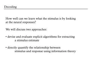
Decoding • How well can we learn what the stimulus is by looking • at the neural responses? • We will discuss two approaches: • devise and evaluate explicit algorithms for extracting • a stimulus estimate • directly quantify the relationship between • stimulus and response using information theory
Reading minds: the LGN Yang Dan, UC Berkeley
Two-alternative tasks Britten et al. ‘92: behavioral monkey data + neural responses
Predictable from neural activity? Discriminability: d’ = ( <r>+ - <r>- )/ sr
z p(r|-) p(r|+) <r>+ <r>- Signal detection theory Decoding corresponds to comparing test, r, to threshold, z. a(z) = P[ r ≥ z|-] false alarm rate, “size” b(z) = P[ r ≥ z|+] hit rate, “power” Find z by maximizing P[correct] = p(+) b(z) + p(-)(1 –a(z))
ROC curves summarize performance of test for different thresholds z Want b 1, a 0.
ROC curves: two-alternative forced choice Threshold z is the result from the first presentation The area under the ROC curve corresponds to P[correct]
Is there a better test to use than r? • The optimal test function is the likelihood ratio, • l(r) = p[r|+] / p[r|-]. • (Neyman-Pearson lemma) • Note that • l(z) = (db/dz) / (da/dz) = db/da • i.e. slope of ROC curve
The logistic function If p[r|+] and p[r|-] are both Gaussian, P[correct] = ½ erfc(-d’/2). To interpret results as two-alternative forced choice, need simultaneous responses from “+ neuron” and from “– neuron”. Simulate “- neuron” responses from same neuron in response to – stimulus. Ideal observer: performs as area under ROC curve.
More d’ • Again, if p[r|-] and p[r|+] are Gaussian, • and P[+] and P[-] are equal, • P[+|r] = 1/ [1 + exp(-d’ (r - <r>)/ s)]. • d’ is the slope of the sigmoidal fitted to P[+|r]
Close correspondence between neural and behaviour.. Why so many neurons? Correlations limit performance.
Likelihood as loss minimization Penalty for incorrect answer: L+, L- For an observation r, what is the expected loss? Loss-= L-P[+|r] Cut your losses: answer + when Loss+ < Loss- i.e. L+P[-|r] > L-P[+|r]. Using Bayes’, P[+|r] = p[r|+]P[+]/p(r); P[-|r] = p[r|-]P[-]/p(r); l(r) = p[r|+]/p[r|-] > L+P[-] / L-P[+] . Loss+ = L+P[-|r]
comparing to threshold Likelihood and tuning curves For small stimulus differences s and s + ds
Population coding • Population code formulation • Methods for decoding: • population vector • Bayesian inference • maximum likelihood • maximum a posteriori • Fisher information
Population vector RMS error in estimate Theunissen & Miller, 1991
Population coding in M1 Cosine tuning: Pop. vector: For sufficiently large N, is parallel to the direction of arm movement
The population vector is neither general nor optimal. “Optimal”: make use of all information in the stimulus/response distributions
Bayesian inference By Bayes’ law, likelihood function conditional distribution prior distribution a posteriori distribution marginal distribution
Bayesian estimation Want an estimator sBayes Introduce a cost function, L(s,sBayes); minimize mean cost. For least squares cost, L(s,sBayes) = (s – sBayes)2 ; solution is the conditional mean.
Bayesian inference By Bayes’ law, likelihood function a posteriori distribution
Maximum likelihood Find maximum of P[r|s] over s More generally, probability of the data given the “model” “Model” = stimulus assume parametric form for tuning curve
Bayesian inference By Bayes’ law, likelihood function conditional distribution prior distribution a posteriori distribution marginal distribution
MAP and ML ML: s* which maximizes p[r|s] MAP: s* which maximizes p[s|r] Difference is the role of the prior: differ by factor p[s]/p[r] For cercal data:
Decoding an arbitrary continuous stimulus • Work through a specific example • assume independence • assume Poisson firing Distribution: PT[k] = (lT)k exp(-lT)/k!
Decoding an arbitrary continuous stimulus E.g. Gaussian tuning curves
Need to know full P[r|s] Assume Poisson: Assume independent: Population response of 11 cells with Gaussian tuning curves
Apply ML: maximize lnP[r|s] with respect to s Set derivative to zero, use sum = constant From Gaussianity of tuning curves, If all s same
Apply MAP: maximiseln p[s|r] with respect to s Set derivative to zero, use sum = constant From Gaussianity of tuning curves,
Given this data: Prior with mean -2, variance 1 Constant prior MAP:
How good is our estimate? For stimulus s, have estimated sest Bias: Variance: Mean square error: Cramer-Rao bound: Fisher information (ML is unbiased: b = b’ = 0)
Fisher information Alternatively: Quantifies local stimulus discriminability
Fisher information for Gaussian tuning curves For the Gaussian tuning curves w/Poisson statistics:
Do narrow or broad tuning curves produce better encodings? Approximate: Thus, Narrow tuning curves are better But not in higher dimensions!
Fisher information and discrimination Recall d' = mean difference/standard deviation Can also decode and discriminate using decoded values. Trying to discriminate s and s+Ds: Difference inML estimate is Ds (unbiased) variance in estimate is 1/IF(s).
Limitations of these approaches • Tuning curve/mean firing rate • Correlations in the population