Multiple Regression
Multiple Regression. Advanced Issues. Correlation. Any multivariate technique concerns the relationships among variables Correlation is a measure of the strength and direction of a linear relationship between two variables Two variables’ values vary about their mean (variance)

Multiple Regression
E N D
Presentation Transcript
Multiple Regression Advanced Issues
Correlation • Any multivariate technique concerns the relationships among variables • Correlation is a measure of the strength and direction of a linear relationship between two variables • Two variables’ values vary about their mean (variance) • They may also covary with one another, having the tendency to move in the same or opposite directions (covariance) • As such a correlation is an effect size in and of itself* • When squared it represents the shared variance between the two variables
Linearity Nonlinear relationships will have an adverse effect on a measure designed to find a linear relationship Reliability of measurement If you are not reliably distinguishing individuals on some measure, you will not capture the covariance that measure may have with another adequately Heterogeneous subsamples Sub-samples may artificially increase or decrease overall r. Solution - calculate r separately for sub-samples & overall, look for differences Can be caused by lack of reliability Range restrictions Limiting the variability of your data can in turn limit the possibility for covariability between two variables, thus attenuating r. Common example occurs with Likert scales E.g. 1 - 4 vs. 1 - 9 However it is also the case that restricting the range can actually increase r if by doing so, highly influential data points would be kept out Wilcox 2001 Outliers can artificially increase or decrease r Factors affecting correlation
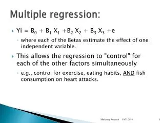
Regression • Using the covariances among a set of variables, regression is a technique that allows us to predict an outcome based on information provided by one or more other variables • We also can get a sense of the overall correlation between a set of variables and some outcome • Multiple R • Squaring that value has the same interpretation as before • Regression equation:
Conceptual Understanding (X1) 1 (X2) 2 Dependent Variable (X3) 3 X’ 4 (X4) New Linear Combination
Interpreting Regression Results: Basics • Intercept • Value of Y if X(s) is 0 • Often not meaningful, particularly if it’s practically impossible to have an X of 0 (e.g. weight) • Slope, the regression coefficient • Amount of change in Y seen with 1 unit change in X • In MR that is with the others held constant • Standardized regression coefficient • Amount of change in Y seen in standard deviation units with 1 standard deviation unit change in X • In simple regression it is equivalent to the r for the two variables • Standard error of estimate • Gives a measure of the accuracy of prediction • R2 • Proportion of variance in the outcome explained by the model • Effect size
Real regression: Starting out • Doing a real regression involves much more than obtaining output • First one must discern the goal of the regression, and there are two main kinds that are for the most part exclusive to one another • Prediction • With prediction there is much less concern over variable importance etc. • One is more concerned with whether it (the model) works rather than how it works • Coefficients will be used to predict future data • Explanation • The goal here is to understand the individual relationships of variables with some outcome • Causal notions are implicit in this approach • Majority of psych usage, and the one that will typically be of focus here
Variable X A Criterion Variable Y B C Variable Z Real regression: Starting out • Specifying the model is obviously something to be done before data collection* unless one is doing a truly exploratory endeavor • However one must consider relations (potentially causal ones) among all the variables under consideration • Given 3 variables of which none are initially set as an outcome, there are possibly 20 or more models which might best represent the state of affairs • In addition one must consider interactions (moderating effects) among the variables • Reliable measures must be used, or it will be all for naught • For some reason people try anyway
Real regression: IED • Initial examination of data includes: • Getting basic univariate descriptive statistics for all variables • Graphical depiction of their distribution • Assessment of simple bivariate correlations • Inspection for missing data and determining how to deal with it* • Start noting potential outliers, but realize that univariate outliers may not be model outliers • The gist is you should know the data inside and out before the analysis is conducted
Real regression: Running the Analysis • ANOVA summary table- you should know every aspect of an ANOVA table and how it is derived • The following is for the simple case, for MR, the Model dF is the number of predictors, the Error df is N- K – 1 • The square root of the MSerror is the standard error of estimate • R2 is the Model SS/ Total SS, the amount of variance explained • All of this is the same for the ‘analysis of variance’
Starting point: Statistical significance of the model The ANOVA summary table tells us whether our model is statistically adequate R2 different from zero The regression equation is a better predictor than the mean As with simple regression, the analysis involves the ratio of variance predicted to residual variance As we can see, it is reflective of the relationship of the predictors to the DV (R2), the number of predictors in the model, and sample size
The Multiple correlation coefficient The multiple correlation coefficient is the correlation between the DV and the linear combination of predictors which minimizes the sum of the squared residuals More simply, it is the correlation between the observed values and the values that would be predicted by our model Its squared value (R2) is the amount of variance in the dependent variable accounted for by the independent variables
Back up • Wait a second what just happened? • You ‘did’ an MR analysis, but how did you do it? • Click the icon • You don’t have to get crazy with it, but you should get a sense of how the data is manipulated to produce coefficients, regular or standardized • You also need to be able to produce the formula a predicted value given the coefficients*
Variable Importance • As the goal of much of social science research is explanation, determining variable importance is a key concern • Unfortunately, the way it is typically done is crude, difficult to make sense of, and not done with much thought • We will go over the standard fare then provide a ‘new’* technique that is highly interpretable and a means to test for differences among variable importance metrics
“Controlling for” • Let’s start with raw coefficients- What do they tell us? • How much does Y change with a one unit change in X… controlling for the other variables in the model • Now for some fun go ask random researchers what ‘controlling for’ actually means • At a conceptual level it simply means we are considering this variable’s effects on the DV with respect to the other predictors • What it actually means is that this is the average effect (slope) seen at each of the levels of the other variables • E.g. average effect of sex role identity on marital satisfaction for each value of age • It does not mean experimental control, and it also doesn’t mean we’ve controlled for what might be potentially important variables that weren’t included in the model
Variable importance: Statistical significance We can examine the output to determine which variables statistically significantly contribute to the model Standard error measure of the variability that would be found among the different slopes estimated from other samples drawn from the same population This is typically not a good way to determine variable importance and should probably only be noted casually if at all However the standard error does allow us to get confidence intervals for the coefficients, which are desirable and should be a standard part of reporting
The standardized coefficient • If we standardized our variables before running the regression analysis (i.e. used the correlation matrices) we would have a standardized regression coefficient • How much Y would typically change given a one standard deviation change in X • In the simple setting it equals the Pearson r, in MR it is a type of partial correlation • We typically prefer this because most of the measures used in psychology are on arbitrary scales (e.g. Likert) • In this manner we can more easily compare one variable to another
Variable importance: Partial correlation Partial correlation is the contribution of a predictor after the contributions of the other predictors have been taken out of both that predictor and the DV A+B+C+D represents all the variability in the DV to be explained (fig. 1 and 2) A+B+C = R2 for the model The squared partial correlation is the amount a variable explains relative to the amount in the DV that is left to explain after the contributions of the other predictors have been removed from both the predictor and criterion It is A/(A+D) (fig. 3) For Predictor 2 it would be B/(B+D) (fig. 4) Figure 1 Figure 2 DV Predictor 1 Predictor 2 Figure 3 Figure 4
Variable importance: Semipartial correlation The semipartial correlation (squared) is perhaps the more useful measure of contribution It refers to the unique contribution of A to the model, i.e. the relationship between the DV and predictor after the contributions of the other predictors have been removed from the predictor in question A/(A+B+C+D) For predictor 2 B/(A+B+C+D) Interpretation (of the squared value): Out of all the variance to be accounted for, how much does this variable explain that no other predictor does? or How much would R2 drop if the variable were removed?
Variable importance Note that exactly how partial and semi-partial will be figured will depend on the type of multiple regression employed. The previous examples concerned a ‘standard’ multiple regression situation As a preview, for sequential (i.e. hierarchical) regression the partial correlation would be Predictor1 = (A+C)/(A+C+D) Predictor2 = B/(B+D) Predictor 1 Predictor 2
Semipartial correlation • For semi-partial correlation • Predictor1 = (A+C)/(A+B+C+D) • Predictor2 same as before • The result for the addition of the second variable is the same as it would be in standard MR • Thus if the goal is to see the unique contribution of a single variable after all others have been controlled for, the results of a sequential regression can be determined to an extent with the squared semipartial correlations from a regular MR • In general terms, it is the unique contribution of the variable at the point it enters the equation (sequential or stepwise)
Variable importance: Example data The semipartial correlation is labeled as ‘part’ correlation in SPSS* Here we can see that education level is really doing all the work in this model
Another example Mental health symptoms predicted by number of doctor visits, physical health symptoms, number of stressful life events
Another example Here we see that physical health symptoms and stressful life events both significantly contribute to the model in a statistical sense Examining the unique contributions, physical health symptoms seem more ‘important’, but unless you run a bootstrapping procedure to provide a statistical test for their difference, you have zero evidence to suggest one is contributing significantly more than the other In other words, that difference my just be due to sampling variability and unless you test that you cannot say that e.g. .381 and .223 are statistically different
Variable Importance: Comparison Comparison of standardized coefficients, partial, and semi-partial correlation coefficients All of them are ‘partial’ correlations in the sense that they give an account of the relationship among a predictor and the DV after removing the effects of others in some fashion
Variable Importance: A more intuitive metric • The problem with all of the previous measures of variable importance is that they don’t decompose R2 into the relative contributions to it from the predictors • There is one that provides an average R2 increase, depending on the order a predictor enters into the model • 3 predictor example A B C; B A C, C A B etc. • One way to think about it using what you’ve just learned is thinking of the squared semi-partial correlation whether a variable is first second third etc. • This statistic is just an average semi-partial, and note that the average is for all possible permutations • E.g. the R-square contribution for B being first in the model includes B A C and B C A, both of which would of course be the same value
As Predictor 1: R2 = .629 Note there are 2 models in which war would be first and have that value (war, math, bush; war, bush, math) Outcome: Score on a Social Conservativism/Liberalism scale As Predictor 2: R2 change = .639 and .087 Here there are two models in which war would be second (math, war, bush; bush, war, math) As Predictor 3: R2 change = .098 There are 2 models in which war would be last and have that value.
Interpretation The average of these* is the average contribution to R square for a particular variable over all possible orderings In this case for war it is ~.36, i.e. on average, it increases R square 36% of variance accounted for Furthermore, if we add up the average R-squared contribution for all three… .36+.28+.01 = .65 .65 is the R2 for the model
Example The output of interest is labeled as LMG below LMG stands for Lindemann, Merenda and Gold, authors who introduced it in a textbook in the early 80s ‘Last’ is simply the squared semi-partial correlation ‘First’ is just the square of the simple bivariate correlation between predictor and DV ‘Beta squared’ is the square of the beta coefficient with all variables in ‘Pratt’ is the product of the standardized coefficient and the simple bivariate correlation It too will add up to the model R2 but is not recommended, one reason being that it can actually be negative lmg last first betasq pratt BUSH 0.278 0.005 0.551 0.024 0.116 MATH 0.012 0.016 0.009 0.016 0.012 WAR 0.363 0.098 0.629 0.439 0.526
Relative Importance Summary There are multiple ways to estimate a variable’s contribution to the model, and some may be better than others A general approach: Check simple bivariate relationships If you don’t see worthwhile correlations with the DV there you shouldn’t expect much from your results regarding the model* Check for outliers and compare with robust measures also You may detect that some variables are so highly correlated that one is redundant Statistical significance is not a useful means of assessing relative importance, nor is the raw coefficient typically Standardized coefficients and partial correlations are a first step Compare standardized to simple correlations as a check on possible suppression Of typical output the semi-partial correlation is probably the more intuitive assessment The LMG is also intuitive, and is a natural decomposition of R2, unlike the others
Multiple Regression: Initial Summary • So far we have gone through some basics of interpreting a MR analysis • However an adequate, responsible MR will have much of the analysis spent testing assumptions, identifying problem cases, determining model adequacy, and validating the model • We turn to that now
How does MR work? • Recall our formula for a straight line in simple regression • Now we have multiple predictors, so the formula will now represent vectors and matrices X here is the dataframe with a column for the constant
How does MR work? • Dimensions of Y = n,1 • Dimensions of X = n, k+1 • Dimensions for the vector of coefficients b = k+1,1 • Dimensions of the vector of residuals e = n,1
How does MR work? • First we need the coefficients • Take the transpose of the data matrix and multiply it by the original datamatrix, as well as the vector of values of the DV • Take the inverse of the first product and multiple that by the second product to obtain the vector coefficients • Multiply the data matrix by the vector of coefficients • The result will be a vector of predicted values • Subtract from the vector of observed to get the vector of residuals
How does MR work? • Another way: • Bi= column vector of standardized regression coefficients • Rii = matrix of correlations among the predictors • Riy = column vector of correlations of the DV and predictors • Ryi = is now the row vector of correlations of the DV and predictors

