Chapter 9 Polynomial Functions
Chapter 9 Polynomial Functions. The last functions chapter. Section 9-1 Polynomial Models. A polynomial in x is an expression of the form where n is a nonnegative integer and The degree of the polynomial is n

Chapter 9 Polynomial Functions
E N D
Presentation Transcript
Chapter 9 Polynomial Functions The last functions chapter
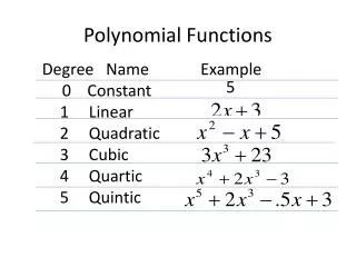
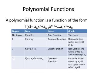
Section 9-1 Polynomial Models • A polynomial in x is an expression of the form where n is a nonnegative integer and • The degree of the polynomial is n • The leading coefficient is • When the exponents are in descending order, the polynomial is in standard form • Ex1. • A) write in standard form • B) what is the degree? • C) what is the leading coefficient?
A polynomial function is one whose rule can be written as a polynomial • A monomial has one term (i.e. 5xyz) • A binomial has two terms (i.e. 5x + 3z) • A trinomial has three terms (i.e. 5x – 3y + 4z) • Open your book to page 558 and look at Ex2. • To find the degree of a polynomial, find the degree of each individual monomial and use the largest number • Ex2. Find the degree of
Section 9-2 Graphs of Polynomial Functions • When discussing the maximum and minimum values, they are speaking in terms of y-values • The maximum and minimum values are known as the extreme values or extrema • Relative extrema are the maximum and/or minimum values within a restricted domain • They are also called the “turning points” of the function • Open your book to page 564 and look at the graphs
The x-intercepts of a function are also known as the roots or the zeros of the function • To find the exact roots of a quadratic function (degree of 2), use the quadratic function and simplified radical form • Otherwise you can use your graphing calculator or factoring to solve • No general formulas for finding the zeros of polynomial functions of degree higher than 4 exist • For functions of degree 3 or 4, graph and use your calculator to find the zeros
A function is considered to be positive on a given interval when the values of the dependent variable (y-values) are positive • A function is considered to be negative on a given interval when the values of the dependent variable (y-values) are negative • A function is said to be increasing on an interval if the slope is positive in that interval • A function is said to be decreasing on an interval if the slope is negative in that interval • Open your book to page 566 and read the example
Section 9-3 Finding Polynomial Models • Ex1. f(x) = 3x + 2 • A) find f(0), f(1), f(2), f(3), and f(4) • B) find the differences between each term (right – left) • Ex2. f(x) = x² + 4x – 6 • A) find f(0), f(1), f(2), f(3), f(4), and f(5) • B) find the first and second differences • A constant difference will occur at the degree of the polynomial (first differences were the same for a linear function, second differences for quadratic function, third differences for a cubic, etc.)
Polynomial Difference Theorem: The function y = f(x) is a polynomial function of degree n if and only if, for any set of x-values that form an arithmetic sequence, the nth difference of corresponding y-values are equal and non-zero • You can use this, along with your calculator to create polynomial models • Read about coefficients and tetrahedral numbers • Ex3. a) find the degree of the polynomial b) find the equation for f(x)
Section 9-4 Division and the Remainder Theorem • Terminology reminder: 100 ÷ 20 = 5 • 100 is the dividend, 20 is the divisor, 5 is the quotient • Use the algorithm for long division of numbers with polynomials • Ex1. (2x² – 9x – 18) ÷ (x – 6) • Ex2. (6x³ – 7x² + 9x + 4) ÷ (3x + 1) • You must show work on these types of questions • If there is a remainder, write it:
The remainder must have a smaller degree than the divisor • Ex3. (4x³ – 4x + 8) ÷ (2x + 6) • If a polynomial, f(x) is divided by x – c, then the remainder is f(c) • Ex4. Find the remainder of • You don’t have to do the division to find the remainder. For example 4, just find f(5)
Synthetic Division (Pre-Calc 4-5) • Another way to divide polynomials is with synthetic division • To use synthetic division, you must write all polynomials in standard form and include all terms • To understand synthetic division, you must first be able to use synthetic substitution • Ex1. Find f(4) for • Synthetic substitution will find the answer to example 1 in another way
Synthetic substitution: • Write the x value to the left • Write the coefficients to each of the terms in order to the right (slightly spaced apart) • Bring down the first coefficient, multiply it by the x value • Write the answer under the next coefficient and add the two together • Repeat until you have used all of the coefficients • The final value is the f(x) value • Ex2. Solve Ex1. using synthetic substitution
Ex3. Use repeated factoring to write the polynomial from Ex1. in nested form • The other numbers below the addition line in Ex2. turn out to be the coefficients to the terms you get when you divide the polynomial by (x – the value) • So using example 1: • Look at the top of page 251 from the Pre-Calc book to see how this looks with variables • This is synthetic division
Use synthetic division to divide • Ex4. • Ex5.
Section 9-5 The Factor Theorem • For a polynomial f(x), a number c is a solution to f(x) = 0 if and only if (x – c) is a factor of f • Factor-Solution-Intercept Equivalence Theorem: For any polynomial f, the following are logically equivalent statements: 1) (x – c) is a factor of f 2) f(c) = 0 3) c is an x-intercept of the graph y = f(x) 4) c is a zero of f 5) the remainder when f(x) is divided by (x – c) is 0
Ex1. Factor • Because a term from example 1 can be factored by 2 (k = 2), that 2 could have been applied to any of the binomials • Ex2. Find two equations for a polynomial function with zeros: • You cannot determine the degree because k is unknown • Open your book to pages 586-587 to see example 2
Section 9-6 Complex Numbers • Imaginary numbers: • Therefore i² = -1 • Ex1. Solve without a calculator • Complex numbers: a + bi where a is the real part and b is the imaginary • The complex conjugate of a + bi is a – bi • Ex2. x = 2 + 3i and y = 5 – 2i • A) find x + y • B) find x – y • C) find xy
If a and b are real numbers, then • Without imaginary numbers, you could only factor the difference of squares (not sum of squares) • Ex3. Factor x² + 100 • Ex4. Write in a + bi form: • Ex5. Solve: x² – 6x + 20 = 0 • Discriminant: b² – 4ac • If the discriminant is: • positive, then there are 2 real roots • negative, then there are 2 complex conjugate roots • zero, then there is 1 real root
Section 9-7 The Fundamental Theorem of Algebra • Fundamental Theorem of Algebra: If p(x) is any polynomial of degree n > 1 with complex coefficients, then p(x) = 0 has at least one complex zero • A polynomial of degree n has at most n zeros • The multiplicity (number of times the same zero occurs for a function) of a zero r is the highest power of (x – r) that appears as a factor of that polynomial • For multiplicity, see Ex1. on page 598
A polynomial of degree n > 1 with complex coefficients has exactly n complex zeros, if multiplicities are counted • Let p(x) be a polynomial of degree n > 1 with real coefficients • The graph of p(x) can cross any horizontal line y = d at most n times • When given a graph, to find the lowest degree possible of the equation, draw a horizontal line where it would hit the graph the highest number of times • That is the lowest possible degree (see page 599)
To verify a number is a zero, plug it in for x and the result should be 0 • If an imaginary number is a zero of a function, so is its complex conjugate • See example 3 part b to see how to find the remaining zeros
Section 9-8 Factoring Sums and Differences of Powers • Ex1. Find all of the cube roots of 64 • Sums and Differences of Cubes Theorems: For all x and y, • These are now factored completely • Ex2. Factor 27c³ – 125d³ • Open your book to page 605 to see how to use the previous theorem for all odd powered functions • Ex3. find all the zeros of 3x³ – 75x
Section 9-9 Advanced Factoring Techniques • Use chunking (grouping) as another way of factoring • Ex1. Factor x³ + 2x² – 9x – 18 • Find common factors to factor out and then use algebra on the remaining terms to simplify • Not all questions will be factored or chunked in the same way • Sometimes (with trinomials) it is helpful to separate the middle term in to two separate terms for factoring
Ex2. Factor 4x² + 4x – 15 • When a polynomial in 2 variables is equal to 0, grouping terms may help you graph it (two separate graphs are created and joined as one) • Ex3. Draw a graph of y² + xy + 3x + 3y = 0
Section 9-10 Roots and Coefficients of Polynomials • For the quadratic equation x² + bx + c = 0, the sum of the roots is -b and the product of the roots is c • Ex1. Find two numbers whose sum is 20 and whose product is 50. Show work. • For the cubic equation x³ + bx² + cx + d = 0, the sum of the roots is –b, the sum of the products of the roots two at a time is c, and the product of the three roots is -d
If a polynomial equation p(x) = 0 has leading coefficient and n roots then p(x) = • For the polynomial equation the sum of the roots is -a, the sum of the products of the roots two at a time is a2, the sum of the products of the roots three at a time is -a3, …, and the product of all the roots is